PyTorch allows the user to build neural networks and evaluate their performance using difference loss methods like MAE, MSE, KL divergence, etc. The Kullback-Leibler or KL divergence loss is used to get the distance between the probabilities of the correct and wrong predictions of the NN model. Furthermore, the KLDivLoss() function is offered by the torch library to get the loss value of the predicted value of the neural networks.
How to Calculate KL Divergence Loss of Neural Networks in PyTorch
Calculating KL divergence loss requires building a deep learning model with neural networks like Sequential or MLP. Train these models on the training data and test them using the unseen data to ensure unbiasedness in model making. Once the models made their predictions, simply check their performances using the KL divergence loss function offered by the torch library.
Head into the process of building the sequential model to get the loss value while training:
Model 1: Using Sequential Neural Network
The sequential model is the deep learning model that uses all the phases or processes in a sequence. This model works efficiently in streaming data like strings, video clips, time series, and many other forms. Additionally, it produces output for each input as it uses a single input and produces one output. To learn how to build the sequential model and calculate the performance, go through the listed steps:
Step 1: Access Python Notebook
First, open the Python development environment using Jupyter or Google Colab Notebook. This guide uses the colab notebook which can be created from the official Google Colaboratory page:

Step 2: Import Libraries
This step is to import the required libraries to build and train the sequential model and plot the results at the end:
import torch
from keras.layers import Dense
from sklearn.datasets import make_circles
from keras.models import Sequential
from matplotlib import pyplot
from numpy import where- The Torch library is used to build the deep learning model and contains different methods to implement it.
- Next, the Keras is a Google-built API that is used to add layers in the neural network architectures.
- Now, scikit-learn or sklearn is a Python library to apply machine learning techniques in the model like splitting of data.
- The Matplotlib library allows the user to build a graphical representation that displays different phases of the model.
- Finally, the NumPy is a well-known Python library to build arrays and here it is used to build the dataset for the model.
Step 3: Building the Dataset
Now, build the dataset for the model so the model can be trained on proper diverse data and then plot it on the screen using the pyplot library:
a, b = make_circles(n_samples=1000, noise=0.1, random_state=1)#using the for loop to split the data in training and testing data
for i in range(2):
samples_ix = where(b == i)       #set the structure of the graph with scatter graphs
pyplot.scatter(a[samples_ix, 0], a[samples_ix, 1])
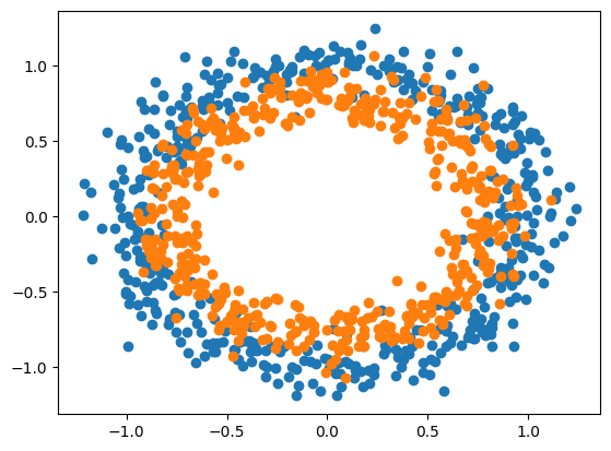
pyplot.show()- Start the make_circles() method to store the 1000 samples in a and b variables with 0.1 noise and random_state to make unbiased data.
- Now, apply the where() method to apply the condition in the for loop to add a condition for splitting data
- Then, call the pyplot library to use the scatter() method to build the scatterplot to get the dataset in two colors.
- To display circles in the graph, use the show() method with the pyplot library:

The color scheme of data shows that data points are stored in two classes in the variables a and b.
Step 4: Splitting the Dataset into Testing and Training Samples
Here, split the data stored in both variables (a and b) into the testing or training data from the complete dataset:
n_test = 500
traina = a[:n_test]
testa = a[n_test:]
trainb = b[:n_test]
testb = b[n_test:]- Start splitting data by creating a variable containing the split value as 500 from the 2000 data samples.
- Both “a” and “b” variables are split into testing and training data containing 500 samples each.
Note: Normalization of Data
After building and splitting the dataset for the model, there is a phase called pre-processing to normalize the dataset. It will be used to remove ambiguities and distortions from the data set in general making it linear for the model. Another process that can be done here is making all the data points in a similar format or structure. This guide did not perform this step as the data set is self-generated and according to the requirements of the model.
Step 5: Building Sequential Model
Now, initialize the model variable with the Sequential() method and then add 100 dimensions of the layers with the activation function. The ReLU activation function is used here to implement the concept of nonlinearity of the model. After that, add sigmoid as the activation function creates an S-shaped curve to predict the class of the final output:
model = Sequential()
model.add(Dense(100, input_shape=(2,), activation='relu'))
model.add(Dense(1, activation='sigmoid'))
Integrate all the components of training and optimizing the sequential model using the compile() method:
model.compile(loss='kl_divergence', optimizer='adam', metrics=['accuracy'])- Call the compile() method with multiple arguments like loss, optimizer, and metrics with all the values.
- Enter the kl_divergence as a value in the loss arguments and the adam optimizer with the accuracy as the metrics.
- Adam optimizer has the advantage of a dynamic learning rate over other optimizers with static LR.
Step 6: Model Fitting
Define the result variable to fit the model for the training of the model and then test it across 30 iterations:
result = model.fit(traina, trainb, validation_data=(testa, testb), epochs=30, verbose=0)- Fitting the model means the training sample from both variables while running the 30 epochs.
- These testing samples are used to validate the accurate performance of the model on the unseen data.
- Now, the verbose is kept 0 here so the model can perform the training in the background to save the computing resources.
Step 7: Model Evaluation
Evaluate the model to get the results of the training and testing data and store them in the train_acc and test_acc variables:
_, train_acc = model.evaluate(traina, trainb, verbose=1)
_, test_acc = model.evaluate(testa, testb, verbose=1)
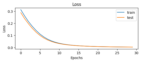
The following snippet displays the loss value for training and testing data which is almost similar and close to zero. Both these aspects are good in the case of machine learning as similar loss values mean that the model is well balanced. A loss value close to zero means that the model is accurate and produces correct answers:

Step 8: Displaying Results
Finally, display the results of the model on the graph for multiple epochs in the training process. Looking at the performance provides us useful insights using the matplotlib library using the following code:
pyplot.subplot(211)
pyplot.title('Loss')
pyplot.plot(result.history['loss'], label='train')
pyplot.plot(result.history['val_loss'], label='test')
pyplot.legend()
pyplot.show()- Display graphs using the subplot(211) to give the graph’s dimensions to represent the loss values of the training and testing data.
- Use the title(‘Loss’) method to display the title of the graph and the plot() method to give the variables (loss and val_loss) from the loss variable.
- Additionally, the plot() method contains the labels for the training and testing lines for better understandability.
- Finally, use the legend() method to give the axis of the graph and the show() method to display the graph:

The results are looking very good as the KL loss value approaches zero making the model accurate. Now, move on to the MultiLayer Perceptron or MLP model using the neural networks of deep learning:
Model 2: Using MLP Neural Network
The MultiLayer Perceptron(MLP) model uses the basic architecture of the neural network as all the neurons are fully connected. It uses the feedforward approach to take the input from the user that keeps moving forward through multiple layers of neurons. The input is extracted from the previous layer’s output to get the final output at the last layer making it the output layer.
To learn the process of building and evaluating the MLP model using the KL divergence loss function, simply go through the following steps:
Step 1: Import Libraries
Get started with the implementation of the model by importing the required dependencies from the torch mentioned below:
import torch #importing torch to get methods for calculating the KL divergence loss
from torch import nn #importing nn dependency to build neural networks
from torchvision.datasets import FakeData #importing FakeData library to get the dataset
from torch.utils.data import DataLoader #importing DataLoader library to load the dataset
from torchvision import transforms #importing transforms library to normalize the data- The torch library offers multiple dependencies like nn to create the neural network models.
- The torchvision library contains different datasets for designing the structure of the neural network models.
- Get the utils library from the torch to get the utility functions like loading the dataset in the model.
Step 2: Configuring MLP Model
Define the MLP class to store the module as the argument with the neural network dependency of the torch:
class MLP(nn.Module): # definition of MLP class with neural network argument

  def __init__(self):# using the constructor of the class to set the structure of the model
    super().__init__()
    self.layers = nn.Sequential(
      nn.Flatten(), #convert multi-dimensional data into 1D
      nn.Linear(28 * 28 * 3, 64), #first layer with its dimensions
      nn.ReLU(), #activation function for the first layer
      nn.Linear(64, 32), #second layer with its dimensions
      nn.ReLU(), #activation function for the second layer
      nn.Linear(32, 1), #third layer with its dimensions
      nn.Sigmoid() #activation function for the last layer
    )

  def forward(self, x): #feedforward approach to set the approach for the model
return self.layers(x)- Create a constructor of the MLP class to configure the architecture of the neural network model.
- Use the Flatten() method to remove all the dimensions and then add the dimensions according to the requirement.
- Apply the Linear(input, output) method to add the dimensions for the input layer with the ReLU() as the activation method.
- The first layer contains the 28 * 28 * 3 input dimension and 64 as the output of the first layer.
- Add the hidden layer with its dimension and then the output layer with the sigmoid() method as the activation function.
- Call the forward() method to apply the feed-forward approach to get the results using all the layers.
Step 3: Building the Dataset
Extract the accurate data using the FakeData() method from the torch library with its arguments and dimensions:
if __name__ == '__main__':
    torch.manual_seed(42)    #extract the data set using the FakeData library from the torchvision
    dataset = FakeData(size=15000, image_size=(3, 28, 28), num_classes=2, transform=transforms.ToTensor())    #load the data set using the DataLoader library from the torch
trainloader = torch.utils.data.DataLoader(dataset, batch_size=64, shuffle=True, num_workers = 4, pin_memory = True)- Firstly, use the manual_seed() method before getting the dataset to apply normalization on the data storage.
- Store the data in the dataset variable using the FakeData() method with the arguments to extract the samples.
- The data contains the 15k samples with (3, 28, 28) dimensions of the image/objects and 2 classes.
- Now, transform the data in the tensors to store the normalized form of data for training the model.
- After that, load the data for training the model in the trainloader variable using the DataLoader() method.
Step 4: Using the KLDivLoss() Function
Integrate all the components configured earlier to store them in their respective variable to be used for training the model:
mlp = MLP()
kl = nn.KLDivLoss()
optimizer = torch.optim.Adam(mlp.parameters(), lr=1e-4)- Start by calling the MLP() method in the mlp variable with the KLDivLoss() function offered by the PyTorch library.
- Now, Adam() is used as an optimizer to get the gradient descent approach using the learning rate as the steps in each iteration.
- Learning rate means that the model evaluates its performance after each epoch and uses it as a head start to improve the accuracy.
- The gradient descent technique is used to fine-tune the parameters of the model after each iteration with the backpropagation approach.
Step 5: Model Training
Use the following code that uses for loop to get three series of iterations with multiple epochs for training the model:
# training the model on the training data so the model can understand the features form the datafor epoch in range(0, 3):
    # printing the iteration number at the start of each iteration with zero loss
    print(f'Starting epoch {epoch+1}')
    current_loss = 0

    for i, data in enumerate(trainloader, 0):      # getting the data and labels from the dataset
      inputs, targets = data
      targets = targets \
                  .type(torch.FloatTensor) \
                  .reshape((targets.shape[0], 1))

      optimizer.zero_grad()
      outputs = mlp(inputs) #getting the predictions using the net variable
      loss = kl(outputs, targets) #getting the loss value by comparing the output and labels
      loss.backward()
      optimizer.step()
      current_loss += loss.item()
      if i % 10 == 0:          # extracting loss values after 10 mini-batches with improvement each time
          print('Loss after mini-batch %5d: %.3f' %
                (i + 1, current_loss / 500)) #printing the epoch number with the loss value after 2000 mini-batches
          current_loss = 0.0

print('\n Training process has finished')- At first, use the nested loop to iterate minibatches in each epoch as the outer loop is used for the epochs.
- The inner loop is used to train the model by providing the input values and extracting the loss value for each iteration.
- The inner loop also contains all the components(Optimizer, loss, model) to train the model with each iteration.
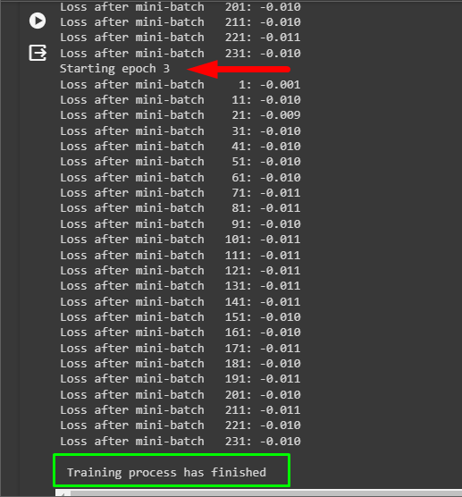
- The if statement is used to get iterations after 10 mini-batches to get an overview of the improvement in the model:

Evaluate the performance of the model by looking at the loss value for each batch in the iteration. The loss value is very near to 0 which tells us that the predictions of the model are accurate.
Conclusion
To calculate the DL Divergence loss of the deep learning model in PyTorch, simply use the KLDivLoss() method or call the compile() method with the loss argument. The user needs to build the Sequential or MLP deep learning model with the neural network architecture to get the predictions. The loss method is then used to evaluate the accuracy and loss values of the neural network model.