Long Short-Term Memory or LSTM is the addition to the Recurrent Neural Network (RNN) by keeping the important previous data. LSTM improves the performance of the Recurrent Neural Network or RNN frequently used with the ordinal data. The ordinal data must be in some meaningful order like text streams in NLP, time-series, DNA sequencing, etc. It works with three gates to identify the important data and send it to the next layer for processing.
The detailed explanation of the LSTM neural network gates is as follows:
Forget Gate is the first gate of the network that identifies the important previous data as the data comes in sequences. It eliminates the non-required or useless data from the stream and keeps the important data only. After that, the remaining previous data is added to the current data, making a complete input for the next gate.
The input Gate is the second gate that takes the input from the forget gate and uses the activation functions. The activation functions are used to train the model so it can understand the important features of the data.
Output Gate is the last gate in the architecture to get the predictions based on the input data. This process uses long-term memory to identify the important information and get accurate predictions:
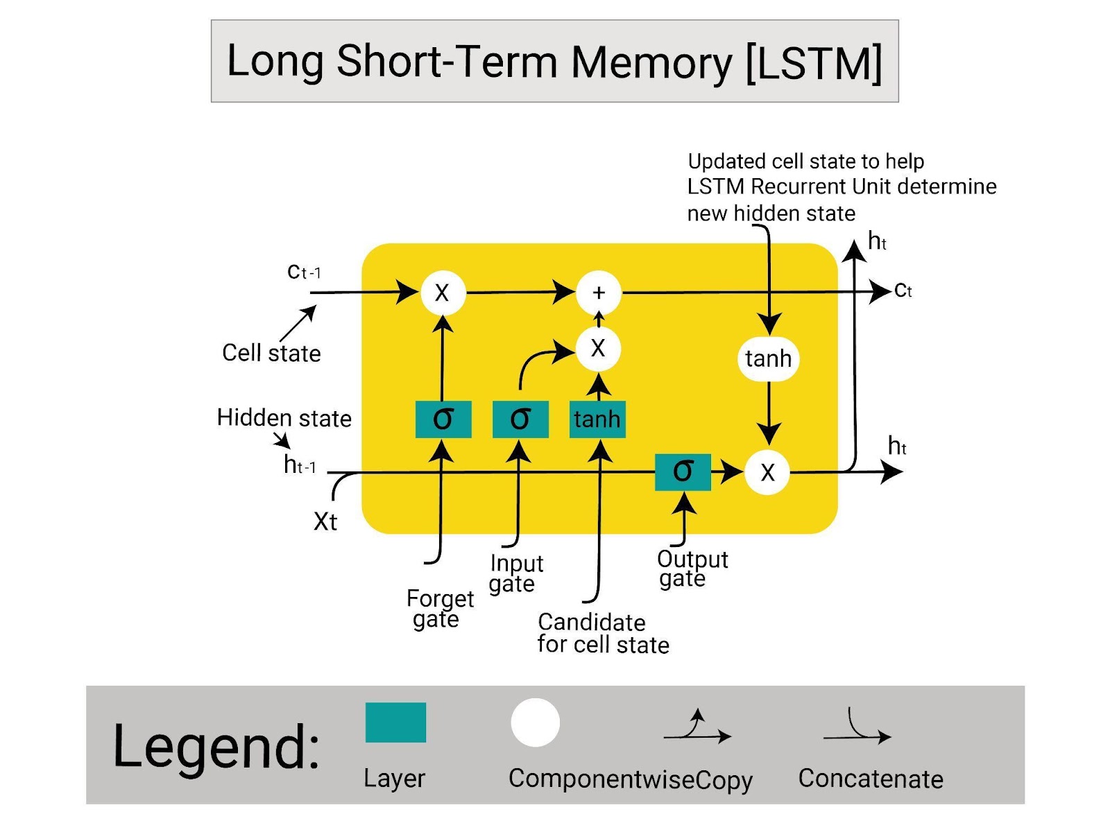
The above picture shows the architecture of the LSTM network with its cell state, hidden state, and gates. The C(t) represents the cell state containing the long-term memory of the network. The h(t) shows the hidden state containing the short-term memory with the important information from the long-term memory.
The important information is extracted by the forget gate and added to the current input in the short memory at the input gate.
How to Design an LSTM Network Using PyTorch
To design the Long Short-Term Memory or LSTM network using PyTorch, get the required libraries to load the sequenced data. After that, preprocess the data to make it applicable to the LSTM network and split the data to train and test the model. Build the structure of the model and then train the model to get the predictions using the input data. To learn how to design the LSTM deep learning model in PyTorch in detail, go through the listed steps:
Step 1: Importing Libraries
First, get the dependencies and functions to build the LSTM neural network by importing the libraries:
import torch
import pandasfrom copy import deepcopy as dc
import numpy
import matplotlib.pyplot as t
import torch.nn as nn from torch.utils.data import Dataset import torch.optim as o- Start by importing the torch library to get the methods of the PyTorch framework.
- Another library required here is pandas to load the dataset as the data frames in Python notebook.
- After that, get the deepcopy library form copy to create copies of the entire objects with their separate address.
- Import the NumPy library to store the data in the form of arrays in Python language.
- Use the matplotlib library to get the pyplot API to display results using graphical representations.
- Get the nn dependency from the torch library to get the methods for neural networks.
- Use the utils dependency to use the datasets provided by the torch library.
- Finally, get the optim dependency from the torch library to use the optimizers.
Step 2: Extracting Dataset
Now, download the original dataset from the Kaggle library and its cleaned version can be downloaded from here. After downloading the dataset, simply upload the dataset in the folder of the Python notebook:
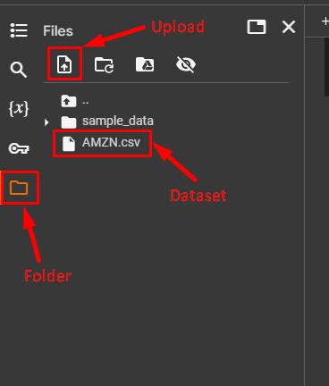
The dataset contains the historical stock prices with the opening and closing prices of each date. It contains more than 6500 days of data with multiple features as well, represented in multiple columns.
Now, use the following code to read the dataset as the data frames and get the required fields:
data = pandas.read_csv('AMZN.csv') #Loading dataset using the pandas' data frame
data = data[['Date', 'Close']]
data- Create the data variable to store the data frames using the read_csv(‘AMZN.csv’) method.
- Use the data variable to show the required fields from the dataset like Date and Close:
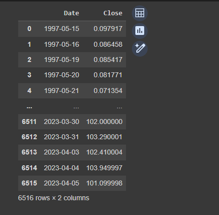
The above screenshot displays the 6516 rows in total with only specific columns asked in the above code.
Step 3: Making the Required Dataset
The LSTM model requires historical data like a series like current data and the data of its previous days. Let’s convert the dataset in the format required to train the LSTM model using the following code:
def prepared_data(df, n_steps):
    df = dc(df) #deepcopy to make a separate copy of the dataset
    df.set_index('Date', inplace=True) #Get the column name as the index to use it as the reference point

    for i in range(1, n_steps+1):
        df[f'Close(t-{i})'] = df['Close'].shift(i) #make a series of the data frames by getting its previous data
    df.dropna(inplace=True)
    return df
#set the lookback number to get the historical data for the index column
lookback = 7#prepared_data() method calling
alter = prepared_data(data, lookback)
#printing the values stored in the variablealter- Define the prepared_data() method with data frames(df) and the number of steps(n_steps) arguments to prepare the data.
- After that, create a copy of the data frame using the deepcopy() method and convert its Date feature.
- Now, use the for loop to get the close value for the current date and its previous 7 days using the lookback variable.
- Create the “alter” variable to store the converted data frame and show the current date with the previous week’s data:
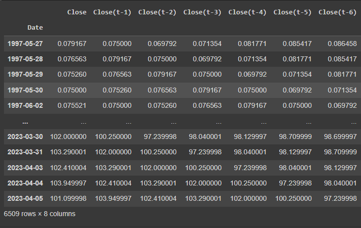
The above screenshot displays that the data is diverse ranging from 0 to over 100 and it needs to be normalized.
Step 4: Preprocessing Dataset
Now, use the converted dataset from the alter variable and store it in the form of arrays using the NumPy library:
from sklearn.preprocessing import MinMaxScaler #library to scale data
alter_np = alter.to_numpy() #storing the data in NumPy arrays
scaler = MinMaxScaler(feature_range=(-1, 1)) #normalize the data within -1 to 1 range
alter_np = scaler.fit_transform(alter_np) #transform to combine all the data- Import the MinMaxScaler library from scikit_learn’s preprocessing dependency to normalize the data.
- After that, create a new variable called alter_np using the to_numpy() method to store the data frames in the form of arrays.
- Use the MinMaxScaler() method to convert the values of the close feature within the range of -1 to 1.
- Use the transform() method using fit dependency to combine the scaled data with the date column in the alter_np variable.
Step 5: Splitting Dataset
Here, store the data from the array in two variables x and y using the following code to split the main dataset:
X = alter_np[:, 1:]
y = alter_np[:, 0]- Initialize the x variable with all the columns except the first column in the data set using the [1:] index.
- Store the first column of the dataset in the variable “y” splitting the dataset into two variables.
- This process is commonly used to prepare the data for the machine learning algorithm to make output(y) and features(x) samples:
Now, use the x and y variables containing the complete data to split the dataset into training and testing samples:
#make the copy of the dataset in its reversed orderX = dc(numpy.flip(X, axis=1))
split_index = int(len(X) * 0.95)
#split the features of the data in the training and testing data
X_train = X[:split_index]
X_test = X[split_index:]
#split the output column of the data in the training and testing data
y_train = y[:split_index]
y_test = y[split_index:]- Create a copy of the array using the deepcopy() method using its alias dc and store it in the x variable.
- define the split_index variable storing 95% of the complete data using the len() method.
- Store 95% of the data as the training data for both(x,y) variables and the rest as the test data.
Here, it is a requirement to build the LSTM in PyTorch to add another dimension to the training and test dataset. Use the following code with the reshape() method train to add dimensions with all the variables:
X_train = X_train.reshape((-1, lookback, 1)) #add a dimension using lookback
X_test = X_test.reshape((-1, lookback, 1)) ))
y_train = y_train.reshape((-1, 1)) #add a dimension to the train and test variable
y_test = y_test.reshape((-1, 1))
Finally, complete the preprocessing step by storing the training and testing data in PyTorch tensors using the following code:
X_train = torch.tensor(X_train).float()
y_train = torch.tensor(y_train).float()
X_test = torch.tensor(X_test).float()
y_test = torch.tensor(y_test).float()
X_train.shape, X_test.shape, y_train.shape, y_test.shape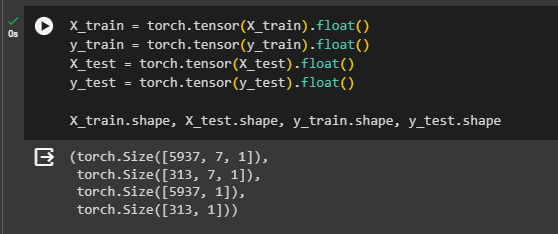
The above screenshot displays the data stored in the tensors with extra dimensions at the end. The training set of “X” and “y” variables contains 6183 rows and the test data contains 326 rows.
Step 6: Combining the Dataset
Now, combine all the columns stored in the x and y to make a complete dataset of training and testing samples:
class TimeSeriesDataset(Dataset):
    def __init__(self, X, y):
        self.X = X
        self.y = y
    #getting the length of the data to make it as streaming data
    def __len__(self):
        return len(self.X)
    #getting the data points of the dataset to store the complete data as a stream
    def __getitem__(self, i):
        return self.X[i], self.y[i]
#store the streaming data set by calling the class
train_dataset = TimeSeriesDataset(X_train, y_train)
test_dataset = TimeSeriesDataset(X_test, y_test)- Create a class named TimeSeriesDataset with the Dataset library as its argument.
- Use the constructor to initialize the X and y variables with the self as an instance of the class.
- Define the len() method to find the length of the data and the getitem() method to return the complete data.
- Finally, initialize the train_dataset and test_dataset variables with the TimeSeriesDataset() class with arguments.
Step 7: Loading the Data
After getting the dataset in the format required to train the model, simply load the dataset using the following code:
from torch.utils.data import DataLoader
#Loading the training and testing dataset using the DataLoader
train_loader = DataLoader(train_dataset, batch_size=16, shuffle=True)
test_loader = DataLoader(test_dataset, batch_size=16, shuffle=False)- Import the DataLoader library from the utils dependency to load the datasets.
- Define the train_loader and test_loader variables to call the DataLoader() method with its arguments.
- Use the first argument as variables containing the dataset and then set the size of the batch at 16 to train the model.
Use the for loop to set the structure of using the batches while training the model to predict the accurate output:
for _, batch in enumerate(train_loader):
    X_batch, y_batch = batch[0], batch[1]
    print(x_batch.shape, y_batch.shape)
break- Use the train_loader variable in the for loop to set the batches(x, y) for giving the input as batch[0] and batch[1] as output.
- After that, print the shape of both batches before breaking out of the loop.
Step 8: Building the LSTM Model
Build the structure of the Long Short-Term Memory model in Pytorch by building its class as mentioned in the following code:
class LSTM(nn.Module):
    def __init__(self, input_size, hidden_size, num_stacked_layers):
        super().__init__()
        self.hidden_size = hidden_size
        self.num_stacked_layers = num_stacked_layers
        #setting the structure of the neural network using stacked layer
        self.lstm = nn.LSTM(input_size, hidden_size, num_stacked_layers,
                            batch_first=True)
        #complete the structure of deep learning with a fully connected layer
        self.fc = nn.Linear(hidden_size, 1)
    #set the feed-forward technique to train the model
    def forward(self, x):
        batch_size = x.size(0)
        h0 = torch.zeros(self.num_stacked_layers, batch_size, self.hidden_size)
        c0 = torch.zeros(self.num_stacked_layers, batch_size, self.hidden_size)
        #get the output from the LSTM model using the hidden and current data
        out, _ = self.lstm(x, (h0, c0))
        out = self.fc(out[:, -1, :])
        return out

model = LSTM(1, 4, 1)- Define the LSTM class with its neural network Module and then define its constructor.
- Initialize the arguments of the constructor in its body to set the structure of the LSTM model.
- The argument contains the layers of the model like input, output, and stacked layer.
- The stacked layer is added here to make the model more deeper so it can predict more accurately.
- It also adds the fully connected layer at the end using the Linear() model to get the final output.
- After that, define the forward() method to set the structure of the LSTM using the current and previous inputs.
- Initialize the h0 variable containing the hidden state suggesting the previous data in the stream.
- Define another variable as c0 to store the current input from the data and apply the lstm() method to them.
- After that, process the inputs and return the prediction value in the out variable.
- Call the LSTM(1, 4, 1) class with arguments suggesting one input layer, four hidden layers, and 1 output layer.
Step 9: Setting the Hyperparameters
The hyperparameters of the model are the parameters that can be set or configured from external sources. Before training the model, set up the hyperparameters of the model to improve the performance of the model:
learning_rate = 0.001
num_epochs = 10
loss_function = nn.MSELoss()
optimizer = o.Adam(model.parameters(), lr=learning_rate)- The first parameter is learning_rate which is set to 0.001 which improves the performance of the model using an optimizer.
- The num_epochs are set to provide the number of iterations for training the model.
- loss_function variable is initiated with the MSELoss() to evaluate the loss value of the model.
- The optimizer variable uses the Adam() method with the model’s parameters using the learning rate.
Step 10: Model’s Training
After that, train the model using the following code to get the loss value of each training iteration:
def train_one_epoch():
    model.train(True)
    print(f'Epoch: {epoch + 1}')
    running_loss = 0.0
    #Training phase of the model using its batches from the training data
    for batch_index, batch in enumerate(train_loader):
        x_batch, y_batch = batch[0], batch[1]
        #store the predictions in the output from the input training data
        output = model(x_batch)
        loss = loss_function(output, y_batch)
        running_loss += loss.item()
      #optimizing the performance by improving the accuracy and minimizing the loss
        optimizer.zero_grad()
        loss.backward()
        optimizer.step()
        #print the loss values of the training set for each iteration
        if batch_index % 100 == 99:
            avg_loss_across_batches = running_loss / 100
            print('Batch {0}, Loss: {1:.3f}'.format(batch_index+1,
                                                    avg_loss_across_batches))
            running_loss = 0.0
print()- Define the train_one_epoch() method with the train() method as true to start the training process.
- Use the for loop with the train_loader variable as the argument and get both batches from the dataset.
- Initialize the output variable with the model() method containing the features of the dataset.
- Get the loss value using the loss_function() method with the output and y_batch variables.
- Apply the gradient descent while backpropagating the LSTM model using the backward() method.
- Use the conditional statement to print the average loss value after 100 iterations.
Define another function named validate_one_epoch() method to test the model by keeping the False value in the train() method:
def validate_one_epoch():
    model.train(False)
    running_loss = 0.0
    #Testing phase of the model using its batches from the test data
    for batch_index, batch in enumerate(test_loader):
        x_batch, y_batch = batch[0], batch[1]
        #optimizing the performance by minimizing the loss
        with torch.no_grad():
            output = model(x_batch)
            loss = loss_function(output, y_batch)
            running_loss += loss.item()

    avg_loss_across_batches = running_loss / len(test_loader)

    print('Val Loss: {0:.3f}'.format(avg_loss_across_batches))
    print('***************************************************')
print()- Use the for loop in the validate function to get the predictions and loss value from the unseen data.
- Get a single loss value for each iteration as the validation loss after calculating the average loss.
Run the loop using the number of iterations to call both the methods like train_one_epoch() and validate_one_epoch():
for epoch in range(num_epochs):
    train_one_epoch()
    validate_one_epoch()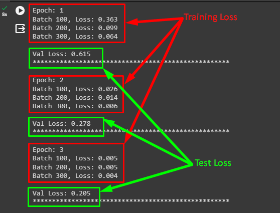
The above screenshot displays the loss values for multiple training batches and then the validation loss for each iteration. The loss value decreases with each iteration showing that the model’s performance is improving and giving better accuracy.
Step 11: Plotting the Results
Finally, display the predicted values compared to the actual values with the line graph using the following code:
with torch.no_grad():
    predicted = model(x_train).to('cpu').numpy()

t.plot(y_train, label='Actual Rate')
t.plot(predicted, label='Predicted Rate')
t.xlabel('Day')
t.ylabel('Rate')
t.legend()
t.show()- Calculate the gradient descent of the predicted values using the no_grad() method.
- Use the plot() method to get the actual and predicted values using their variables and labels.
- Set the xlable() and ylabel() methods to set the titles for the x and y-axis of the graphs.
- Use the legend() method to get the graph and the show() method to display it on the screen.
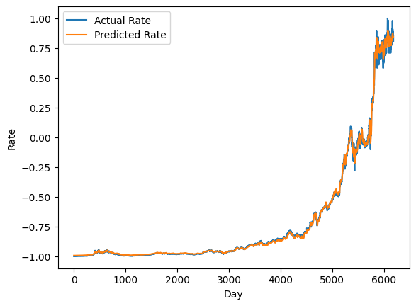
The above screenshot displays the orange line as the prediction values and the blue lines for the actual data. Both the actual and predicted lines are almost aligned as displayed in the above screenshot. It means that the model’s performance is very good and accurate with a minor loss value.
That’s all about how to create and design the structure of the Long Short-Term Memory network using the PyTorch framework.
Conclusion
To design the Long Short-Term Memory or LSTM network using the PyTorch framework, import the required libraries. After that, download and preprocess the dataset to make it according to the requirement of the model. The dataset for the LSTM model should be in a sequential format like a time series and train the model on the data. Finally, test the model to evaluate its performance using the loss value or plot its values using the line graph.