PyTorch is a framework containing dependencies and libraries to build deep learning models. Deep Learning (DL) models use the neural network architecture to predict the future based on historical data. The historical data is authentic so it can be used to evaluate the performance of the model with the loss value using built-in loss functions. PyTorch also allows the user to customize their loss function according to the requirements
Outline
- What is a Custom Loss Function
- How to Design a Custom Loss Function in Deep Learning Models
- Advantages of Custom Loss Functions
What is a Custom Loss Function
A custom loss function allows the user to calculate the wrongly predicted values according to their problem. To do so, the user needs to understand the problem at hand like regression, classification, clustering, or others. By understanding the problem, it becomes easy to design the customized loss function or even use the built-in ones effectively. Now let’s understand how to design a custom function using the PyTorch framework to enhance deep learning models.
The following is the syntax to define a basic customized loss function in the PyTorch framework:
import torch def custom_loss(inp, out):
    loss = torch.mean((out - inp)/ out)
return loss- Import the torch library to get the functions required to build the loss function.
- Now, define the loss function followed by the name(custom_loss) of the function with the input(inp) and output(out) as arguments.
- Here, the “inp” variable contains the historical data, and the “out” stores the predicted data.
- After that, provide the formula in the body to calculate the loss value using its variable.
- Finally, return the loss value or the variable containing the loss values extracted from the formula
Call the custom_loss() function with the arguments to calculate the loss values while training the model.
How to Design a Custom Loss Function in Deep Learning Models
To build the deep learning model with the customized loss function, simply build or extract a dataset. After that, design and train the deep learning model using the dataset created using the torch library. With the training of the model, design the custom loss function and add it in the process to find the model’s performance.
To learn the process of designing the custom loss function in deep learning models in detail, go through the following steps:
Step 1: Importing Libraries
First, get the dependencies or functions by importing the torch library using the following code:
import torch #building deep learning models using neural networks
import torch.nn as nn #neural network dependency to get multiple methods
import torch.optim as optim #optimizer dependency to get methods like Adam or SGD
import matplotlib.pyplot as p #plot the results in the graphical representations- Import the nn dependency to design neural networks and optim to get the optimizer from the torch library.
- After that, import the pyplot API from the matplotlib library to design the graphs for visual representations.
Step 2: Building Dataset
Now, start building the dataset and store it in the input and output variables using the following code:
inp = torch.rand(10000, 1) * 10 #input values containing the actual data
out = 2 * inp + 1 + torch.randn(10000, 1) #output values containing the labeled data- Create the “inp” variable and initialize it with the rand() method to store values between 0 and 1.
- Here, the second variable is the “out” with random values using the inp variable in the mix as well.
- The out variable uses the randn() method that generates the values with mean=0 and sd=1.
Note: Preprocessing is usually the next step after building the dataset for the deep learning model. However, we have created the data from scratch for the model, so we can skip this step and move forward with the model building. Additionally, this step becomes important when using the existing dataset, extracted from public libraries or built for other models.
Step 3: Designing Neural Networks
After that, build the structure of the neural network model to get the predictions using the given data:
class Model(nn.Module): # class to define Neural Network Model
    def __init__(self): # constructor to initialize the Linear() model
        super(Model, self).__init__()
        self.linear = nn.Linear(1, 1) #Linear model to set the flow of the network

    def forward(self, inp): #Feed-forward technique to start from the input layer
return self.linear(inp)- Create a class named Model with the Module argument from the neural networks.
- In the class, define the constructor’s body with the Linear(1, 1) method with a single input and output value.
- Define a method called forward() to apply the feed-forward technique for training the model.
Step 4: Defining Loss Function
Here, it is time to customize a loss function to evaluate the performance of the model designed in the previous step. Use the following code to define the custom_loss() function in the PyTorch framework:
def custom_loss(output, target): #defining the custom loss function with its method
return torch.mean(torch.abs((target - output) / target))- Define the custom loss function using the def keyword followed by the name of the function(custom_loss).
- After that, get two arguments in the custom_loss() method to get the output value from the original data and the model’s predicted value.
- Use the abs() method from the torch library to get the absolute value (its distance from 0).
- Use the formula from the loss value using the mean() method to get the average loss value for each prediction.
- Finally, return the extracted loss value by calling the customized loss function.
Step 5: Calling the Optimizer
Now, integrate all the components of the model and the optimizer in their variable using the following code:
model = Model()
optimizer = optim.SGD(model.parameters(), lr=0.01) #gradient descent optimizer with learning rate- Create the model variable and initialize it with the Model() class designed in step 3 of this guide.
- It is done to easily train the model and also to avoid the complexities in the process.
- After that, call the SGD() method and store it in the optimizer variable with the arguments of the optimizer.
- The model’s parameters are fine-tuned using the learning rate(lr) value given as the argument:
Step 6: Training the Model
Finally, use the following code to train the model on the given data to get the loss value from the customized function:
num_epochs = 1000
losses = []
for epoch in range(num_epochs):

    predictions = model(inp) #Getting the predictions using the input data
    loss = custom_loss(predictions, out) #calculating the loss value
    optimizer.zero_grad() #applying the gradient descent to improve model
    loss.backward() #backpropagating technique to improve loss value
    optimizer.step()
    losses.append(loss.item()) #add all the loss values in the list

    if (epoch + 1) % 50 == 0:
        print(f'Epoch [{epoch + 1}/{num_epochs}], Loss: {loss.item()}')
print("\nTraining Finished")- Create a num_epochs variable with 1000 values suggesting the number of iterations to train the model.
- The losses variable stores the loss values for each iteration in the form of a list.
- Create a for loop with the number of iterations to get the predictions and loss value of each iteration.
- After that, call the optimizer to apply backpropagation using the zero_grad() method to reduce the loss value.
- Store all the loss values in the losses variable using the append() method.
- Finally, print the epoch number with the loss value after 50 iterations as shown in the following screenshot:
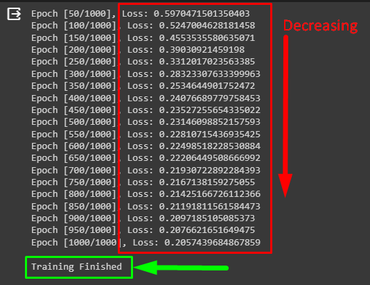
The above screenshot displays that the loss value is decreasing with each training iteration. It means that the model is gradually improving its performance and it ends at 20% after 1000 iterations. To understand it even further, plot the loss values on the graph.
Step 7: Plotting the Loss Value
To represent the values graphically, there are multiple graphs like scatter, bar, or line graphs to display the results effectively. Finally, display the loss values using the line graph by executing the following code:
p.plot(losses)
p.xlabel('Epochs')
p.ylabel('Loss')
p.title('Loss Curve')
p.show()- Call the plot() method with the losses variable containing the loss values for all the training iterations.
- Use the xlabel() and ylabel() methods to give the titles to the x and y-axis on the graph.
- After that, use the title() method to write the name of the graph.
- Finally, use the show() method to display the graph on the screen.
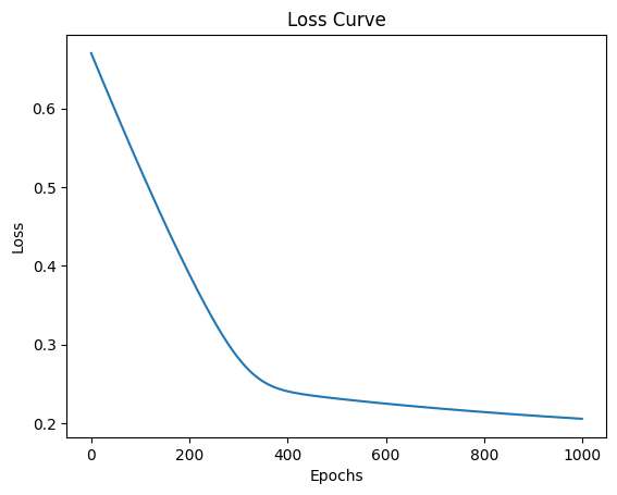
The above snippet shows that the loss value drops suddenly from almost 65% to 25% in 400 iterations. After that, it drops from 25% to 20% in the next 600 iterations suggesting that the model is optimized. If the user wants to improve it further, simply fine-tune the hyperparameters or preprocess the dataset.
Advantages of Custom Loss Functions
Some of the major advantages of building customized loss functions are mentioned below:
- It adds the flexibility aspect as the user has control over the calculating formula for the function and its use.
- Customizing the loss method improves the performance of the evaluation process of the model.
- The user can design a custom loss function to make it compatible with complex models with better accuracy.
That’s all about how to design a custom loss function in deep learning models using PyTorch.
Conclusion
To design the custom loss function in deep learning models using PyTorch, start by building the dataset and normalizing it. After that, design the deep learning model using neural networks to predict the future using the dataset. Then, define the customized loss function to improve the performance of the model using multiple training iterations.