Machine Learning or ML as the name suggests is the way of training or teaching machines to predict the future using the input data from different sources. Deep Learning is the advanced version of the ML models that use the structure of neurons attached to pass on the information from layer to layer. They can automatically improve the performance of the model with multiple iterations and evaluation methods like loss, accuracy, etc.
Quick Outline
This guide explains the following sections:
- What is a Loss Function
- What is Binary Cross Entropy (BCE) Loss
- How to Get BCE Loss of DL Model in PyTorch
- Method 1: Calculate BCE Loss Using the MLP Model
- Method 2: Calculate BCE Loss Using the Keras Library
What is a Loss Function
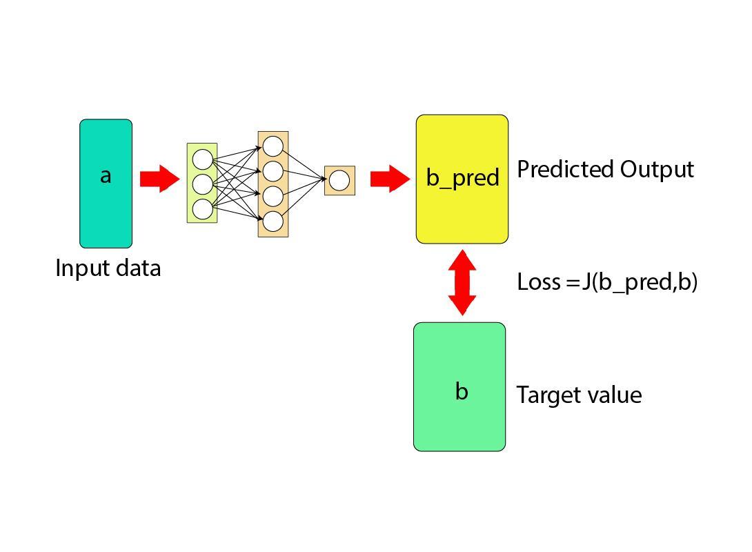
Loss functions are the evaluation techniques to check how the neural networks are performing using the input and predicted values. The input value is given by the user like the historical data that has been considered or proved to be authentic and a fact. The predicted values are the outputs produced by the model and the loss values compare them both to check how accurately the model is performing:

Machine Learning or Deep Learning models are often used to solve problems like regression, classification, or others. In a classification problem, we can not simply find the distance between the actual and predicted values as the classes only have 2 or 3 answers like yes/no, true/false, etc. for millions of rows. To get the loss function for this kind of problem, the Binary Cross Entropy(BCE) loss function is used for optimization.
What is Binary Cross Entropy (BCE) Loss
Binary Cross Entropy or BCE loss values are the summations of the corrected probabilities for the model’s predictions. The BCE loss function will only consider the probability that a model can correct that specific value correctly. After taking the probability of each value in the dataset, the function takes the logarithm of all the instances and then adds them together. The mathematical representation of the Binary Cross Entropy or BCE loss function is as follows:

n: number of rows in the dataset
Ci: Probability of the corrected predictions
The negative sign is attached to the formula as the majority of log values will be negative so the negative value will be converted to the positive:
How to Get BCE Loss of DL Model in PyTorch
Binary Cross Entropy Loss can be used to evaluate the performance of the deep learning models in artificial intelligence. The neural network models are trained multiple times on the same data and the loss value for each iteration provides the improvement index. To learn the process of getting the BCE loss value for the Deep Learning model, simply go through the following methods:
The Google Colab notebook containing the Python code is accessible here:
Method 1: Calculate BCE Loss Using the MLP Model
Multilayer Perceptron or MLP model comes into the light for the Deep learning models using different layers and neurons to predict the future using AI. Perceptron is a logical way of representing the physical structure of the neurons and the neurons are generally structured in multiple layers. To learn the process of implementing the MLP model and optimizing it with BCE Loss in PyTorch, simply follow the steps below:
Step 1: Access Python Notebook
Implementing the Python code requires the creation of a new project using a notebook like Jupyter, VSCode, or Google Colab. This guide uses the Google Colab notebook that can be created by clicking on the “New Notebook” button from the official website:

Step 2: Install Modules
The first line of code is to get the torchmetrics module from the pip Python Package Manager to use its libraries and dependencies:
pip install torchStep 3: Importing Libraries
After getting the module installed, get on with importing the libraries that help in building and training the MLP model. The FakeData library is also required to extract the dataset from the torchvision dependency of the torch and then use its utils dependency to import the DataLoader library:
import os
import torch
from torch import nn
from torchvision.datasets import FakeData
from torch.utils.data import DataLoader
from torchvision import transforms
Step 4: Defining the MLP Model
Build the Multilayer Perceptron neural network using the neural network or nn dependency of the torch library:
class MLP(nn.Module):
  '''
    Neural Network MLP or Multilayer Perceptron
  '''
  def __init__(self):
    super().__init__()
    self.layers = nn.Sequential(
      nn.Flatten(),
      nn.Linear(28 * 28 * 3, 64),
      nn.ReLU(),
      nn.Linear(64, 32),
      nn.ReLU(),
      nn.Linear(32, 1),
      nn.Sigmoid()
    )

  def forward(self, x):
    '''Forward pass through the neurons'''
return self.layers(x)- Define the MLP class with the nn module as the argument to build the deep learning model
- Build the constructor to add the layers in the MLP model with different numbers of neurons and activation functions in each layer
- Define the forward() method to go forward through the layers starting from the first layer towards the output layer.
- The feed-forward approach in neural networks is used to train the model for getting the output with its loss value.
Step 5: Build the Dataset
The following code gets the dataset using the FakeData() method and normalizes it before giving it to the model:
if __name__ == '__main__':
    torch.manual_seed(42)
    dataset = FakeData(size=15000, image_size=(3, 28, 28), num_classes=2, transform=transforms.ToTensor())
trainloader = torch.utils.data.DataLoader(dataset, batch_size=64, shuffle=True, num_workers = 4, pin_memory = True)- Apply the manual_seed() method with the torch library to control the randomness of the data.
- Create the dataset variable to store the data with a 15k size and multiple classes using the FakeData() method
- Define the trainloader variable to call the DataLoader() method to store the dataset for the model.
Step 6: Using the BCELoss() Function
Call the MLP() method in the “mlp” variable and then define the loss_function variable with the BCELoss() method. Set the optimizer for the model using the Adam() method with the optim dependency and the learning rate to train the model:
mlp = MLP()
loss_function = nn.BCELoss()
optimizer = torch.optim.Adam(mlp.parameters(), lr=1e-4)
Step 7: Training & Testing the Model
Now, train the model by running the 3 iterations in mini-batches of 10 per with the loss value displayed for each minibatch:
for epoch in range(0, 3):

    print(f'Starting epoch {epoch+1}')
    current_loss = 0

    for i, data in enumerate(trainloader, 0):
      inputs, targets = data
      targets = targets \
                  .type(torch.FloatTensor) \
                  .reshape((targets.shape[0], 1))

      optimizer.zero_grad()
      outputs = mlp(inputs)
      loss = loss_function(outputs, targets)
      loss.backward()
      optimizer.step()
      current_loss += loss.item()
      if i % 10 == 0:
          print('Loss after mini-batch %5d: %.3f' %
                (i + 1, current_loss / 500))
          current_loss = 0.0

print('\n Training process has finished')- At the start of each iteration, print the starting message with the epoch number
- Run the for loop to train the model in the iterations with the loss value improving in each iteration
- Integrate all the components while training the model like an optimizer, loss, outputs, and others
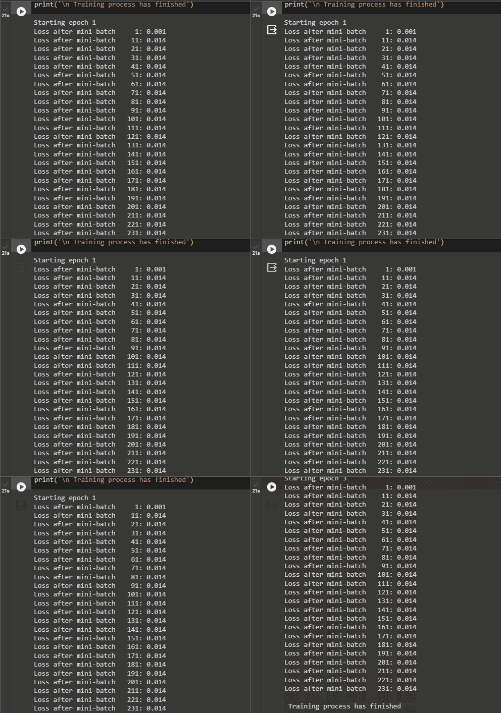
- Increase the current_loss value with each iteration and print its values with the iterations as displayed in the screenshot below:

Method 2: Calculate BCE Loss Using the Keras Library
The Sequential() model is the deep learning model that contains the stack of layers one after the other and the output layer takes the input from the previous layer. The input given to the model at the first layer will go through all the intermediate steps converted as the final output or a prediction of the model. To implement the sequential model and find the loss value using the BCE loss, simply go through the following steps:
Step 1: Import Libraries
The first step here is to import the required libraries like where, Dense, and Sequential for building and training the model. The make_circles library is used to get the data set for training the model and pyplot is used to display the graphical representation of the results:
from keras.layers import Dense
import torch
from sklearn.datasets import make_circles
from numpy import where
from keras.models import Sequential
from matplotlib import pyplot
Step 2: Building the Dataset
After getting the libraries, use the make_circles() method to build the data set of 1000 instances as the sample dataset. Store the dataset in two variables like a and b as different classes and plot the scatter graph using the pyplot library with the show() method:
a, b = make_circles(n_samples=1000, noise=0.1, random_state=1)
for i in range(2):
samples_ix = where(b == i)
pyplot.scatter(a[samples_ix, 0], a[samples_ix, 1])
pyplot.show()
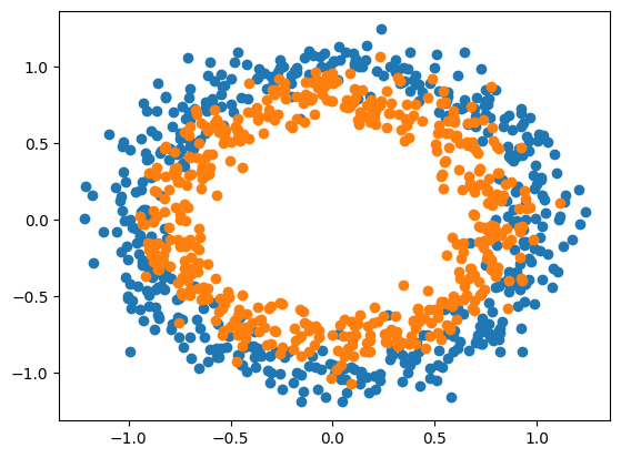
The following picture displays the scatter graph divided into two variables using different colors for the samples:

Step 3: Building the Model
Now, split the dataset into training and testing samples for both a and b variables by setting the size of the training sample. Take half of the sample to make the training set and the other half for the testing set for both classes and store them in multiple variables:
n_test = 500
traina = a[:n_test, :]
testa = a[n_test:, :]
trainb = b[:n_test]
testb = b[n_test:]
Configure the model variable by calling the Sequential() method and then add the neural networks from the model using the Dense() method. After that, add another neuron for the output layer with the sigmoid activation function which gets the input from the previous layer and produces the final result:
model = Sequential()
model.add(Dense(100, input_shape=(2,), activation='relu'))
model.add(Dense(1, activation='sigmoid'))
Step 4: Training the Model
Call the compile() methods with the model variable to provide the evaluation metrics like loss, accuracy, and the adam optimizer. The loss value will be calculated using the binary_crossentropy function from the torch library in the Python language:
model.compile(loss='binary_crossentropy', optimizer='adam', metrics=['accuracy'])Train the model by using the fit() method with all the testing and training sets created in the previous step. With that, provide the number of iterations required to train the model using the epochs argument in the fit() method. The verbose argument is used to display the backend processes for each iteration on the screen:
| result = model.fit(traina, trainb, validation_data=(testa, testb), epochs=300, verbose=0) |
Now, evaluate the model by displaying the loss and accuracy after 300 iterations by setting the verbose argument to 1 and 0 means that the processes won’t be visible:
_, train_acc = model.evaluate(traina, trainb, verbose=1)#Model evaluation using the training and testing variables
_, test_acc = model.evaluate(testa, testb, verbose=1)
The following screenshot displays the loss and accuracy values for the training and testing datasets of both classes:

Step 5: Plotting the Results
After getting the results for the training and testing data, simply plot the values on the screen using the line graph:
pyplot.subplot(211)
pyplot.title('Loss')
pyplot.plot(result.history['loss'], label='train')
pyplot.plot(result.history['val_loss'], label='test')
pyplot.legend()
pyplot.show()- Set the dimensions of the graph by providing the values in the subplot() method
- Set the title of the graph which will be displayed at the top of the visualization
- Give the loss values for the training and testing data using the plot() method
- Finally, display the graph on the screen using the legend() and show() method
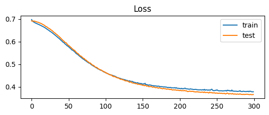
The following screenshot displays the variation in the loss values for both variables throughout the 300 epochs. The loss value drops for both the data starting from 70% to below 40% at the time of the 300th iteration:

Another metric to evaluate the model’s performance is accuracy and the following code is used to plot the graph for testing and training data:
pyplot.subplot(212)
pyplot.title('Accuracy')
pyplot.plot(result.history['accuracy'], label='train')
pyplot.plot(result.history['val_accuracy'], label='test')
pyplot.legend()
pyplot.show()
The accuracy has increased with each iteration as the line goes from 0 to above 80% at the time of 300 iterations:

That’s all about getting the binary cross-entropy loss for deep learning models in PyTorch.
Conclusion
To get the Binary Cross Entropy or BCE Loss from the trained deep learning model, import the required libraries and build the deep learning models. The deep learning or neural network models can be built using the nn dependency of the torch library. After that, test the model and evaluate its performance by finding the BCE loss value for each iteration. This guide has elaborated on evaluating the performance of deep learning models like MLP and sequential.