The absolute value of any real number is its distance from the zero on the number line. It is related to the magnitude or distance, which is always positive. So we can say that an absolute value is the magnitude of the real number, irrespective of its signs.
Why We Need Absolute Values in Google Sheets
Suppose, you want to calculate the distance between -3 and 4. We will calculate the distance between -3 and 0 and then from 0 to 4, we will get 7 by adding both. But if we first get the absolute value of -3 which is its distance from 0 that is 3 then add it to 4, we will get the answer as 7.
But when dealing with large data, it is hard to remove the sign from all negative entries one by one to get their absolute values. Google Sheets helps us in this scenario, as there are very useful formulas to apply to large data collectively to get their absolute values.
How to Find Absolute Value in Google Sheets
There are different useful formulas to apply to large data in Google Sheets to find the absolute values of all the entries collectively. Following is a list of all the methods to find absolute values in Google Sheets. We will discuss them one by one.
- Finding Absolute Values Using ABS() Function
- Removing Negative Signs Using the IF() Function in Google Sheets
- Use Apps Script to Find Absolute Values in Google Sheets
- Find Absolute Values Using Power Tools Feature In Google Sheets
Method 1: Finding Absolute Values Using ABS() Function
The ABS() function, in Google Sheets, converts all the negative entries from the selected data without affecting the positive entries. The syntax used for the ABS() formula is as follows,
ABS(value)Where value is the argument used for reference to the cell to which we would like to find the absolute value.
To better understand the use of the ABS() formula, follow the following steps by taking an example of small-size data in Google Sheets.
Step 1: Click on an empty cell in Google Sheets, then type =ABS(A3).
Here, A3 is the value argument used for the reference of the first cell containing a number in the data.
Now, press Enter, and we will get the absolute value of the number in the A3 cell:
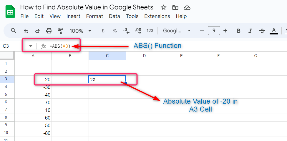
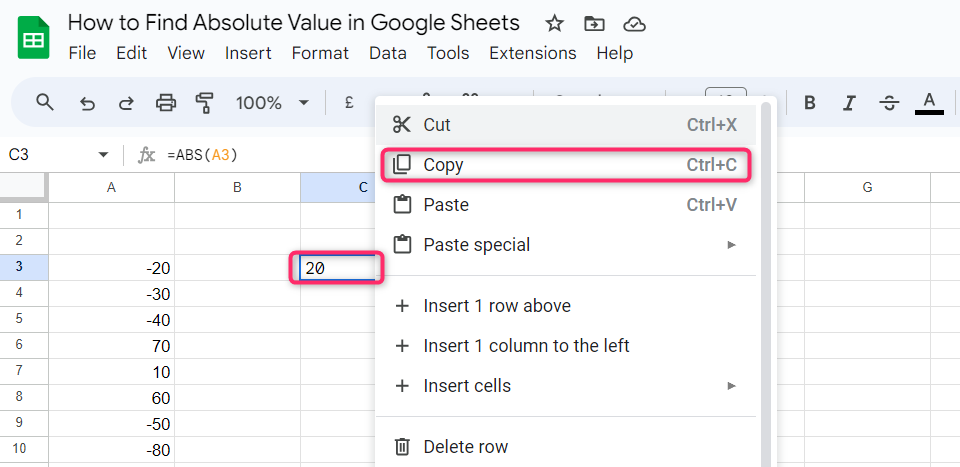
Step 2: Right-click the same cell and click on Copy from the context menu:
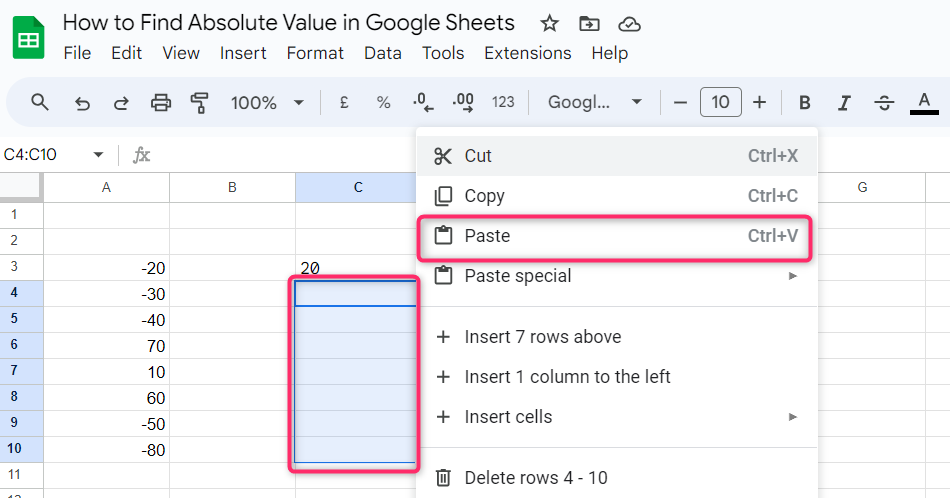
Step 3: Click on the next cell and move the cursor down to select more cells equal to the cells containing the data. Right-click on the selected cells and click on Paste from the context menu:
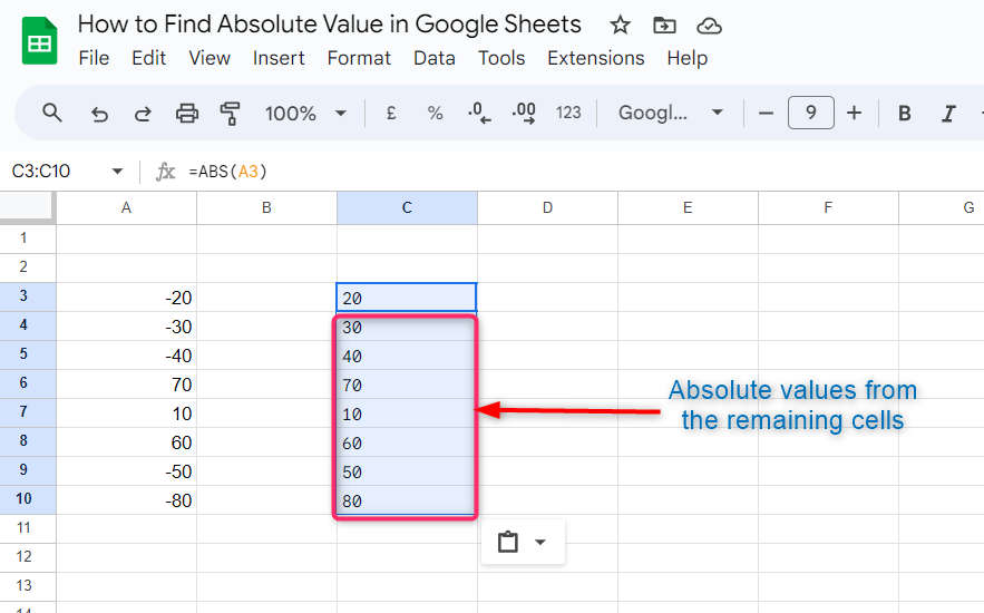
Step 4: As soon you paste the function on the selected cells, you will get the absolute value of all the entries in the same order they are arranged in the data cells:
Method 2: Removing Negative Signs Using the IF() Function in Google Sheets
The IF() function in Google Sheets uses logical expressions, on the basis of which it gives you the result in return. It tests all the entries from the data against the condition you defined in the function, then returns with a result on the basis of the conditions applied.
The following is the syntax used for the IF() function in Google Sheets:
IF(logical_expression, value_if_true, value_if_false)Where
logical_expression is the argument used for the reference to the cell containing an expression representing a logical value.
value_if_ture is the value you will get in return if the logical expression is true.
value_ifP_false is the value you will get in return if the logical expression is false.
To better understand the workings of the IF() function and its arguments, we will apply it step by step to the previous example.
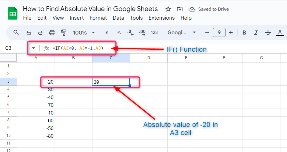
Step 1: Click on the empty cell in the Google Sheets and type =IF(A3<0, A3*-1, A3).
Here,
A3<0 is the logical expression with reference to the A3 cell that contains a value less than zero.
A3*-1 is the value we will get in return if the logical expression is true.
A3 is the value we will get in return if the logical expression is false.
Now press Enter, if there is a number less than zero in the A3 cell it will be multiplied by -1 and return with a positive value, and if the is not less than zero then it will remain the same:
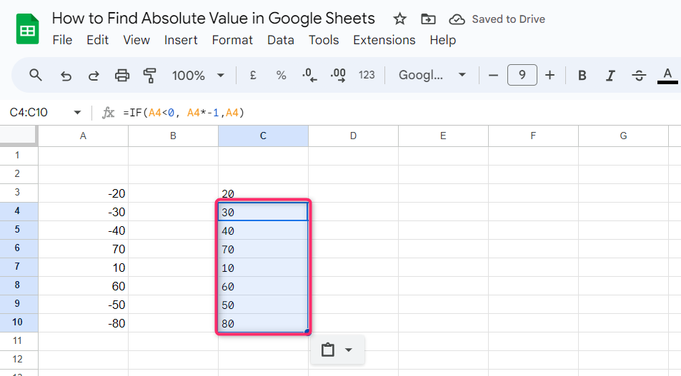
Step 2: Click on the same cell and copy the function applied to that cell, then paste it after selecting the cells equal to the cells containing the data as mentioned in the previous method. We will get the values in return without negative signs, which are absolute values:
Method 3: Use Apps Script to Find Absolute Values in Google Sheets
Apps Script is the coding language that is designed to do more actions in Google applications like Sheets, Docs, Drive, calendar and more.
In Google Sheets, we can apply an Apps Script to large data, and find the absolute values.
Apps Script in Google Sheets helps in finding the absolute values on large-size data quickly. This works on the original data, and we don’t need to click on any empty cell in the Google Sheets to type a formula and paste it to all the cells, as we do in previous sections.
We just select the data and apply Apps Script to it, we will get the absolute value of all the entries in the same cells where they are actually placed.
We can use the following Apps script in Google Sheets to find the absolute values:
function findAbsolute() {
  var app=SpreadsheetApp;
  var ss=app.getActiveSpreadsheet();
  var activeSheet=ss.getActiveSheet();
  var range=activeSheet.getActiveRange();
  var values=range.getValues();
  var value;
  for (var i in values){
    var row=values[i]
    for (var j in row) {
      value=row[j]
      if (value<0){
        row_num=parseInt(i)+1;
        col_num=parseInt(j)+1;
        console.log(value)
        console.log(row_num, col_num)
        activeSheet.getRange(row_num+1,col_num).setValue(value*(-1));
      }
    }
  }
}
We will learn the use of Apps script in Google Sheets step by step by applying it to the previous example.
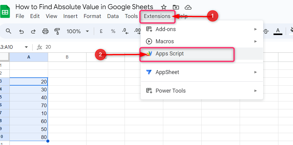
Step 1: Click on the Extensions from the taskbar, then click on Apps Script:
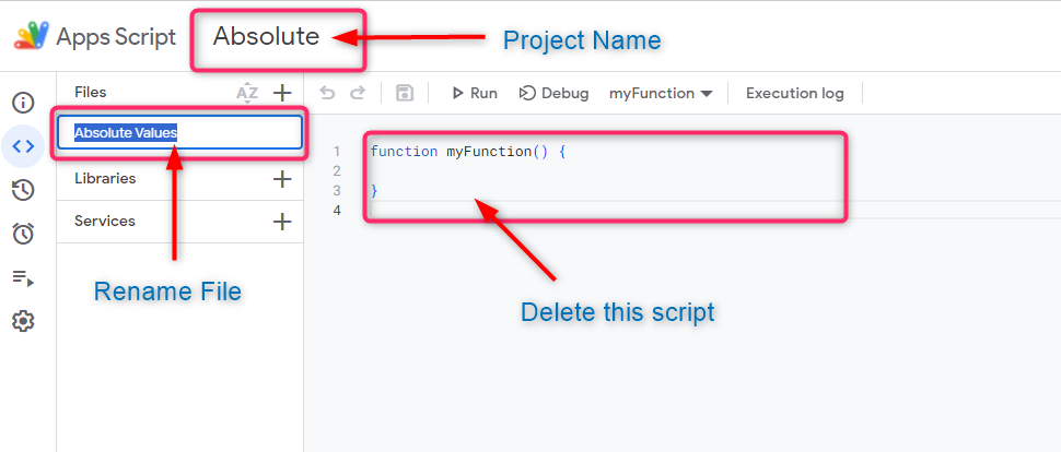
Step 2: Rename the file and project name and delete the already written script:
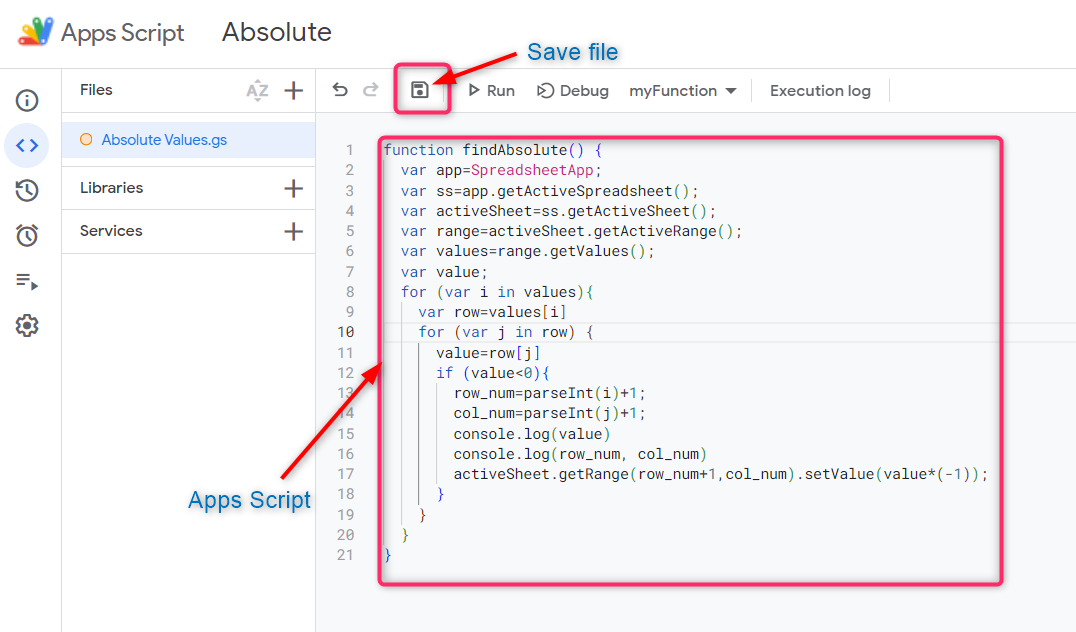
Step 3: Copy the above-mentioned script and paste it into the script section, then save it:
Step 4: Go back to the Google Sheet and again click on the Extensions from the taskbar. In the context menu, click on Macros and click on Import macro in the next menu:
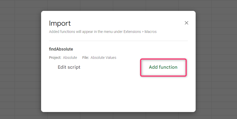
Step 5: Click on Add function in the next window:
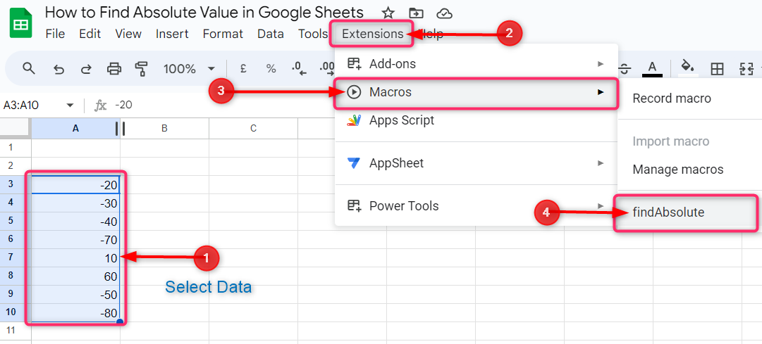
Step 6: Now select the data from which you want to find the absolute values, then click on Extensions and Macros in the context menu. In the macros’ dropdown menu, click on findAbsolute:
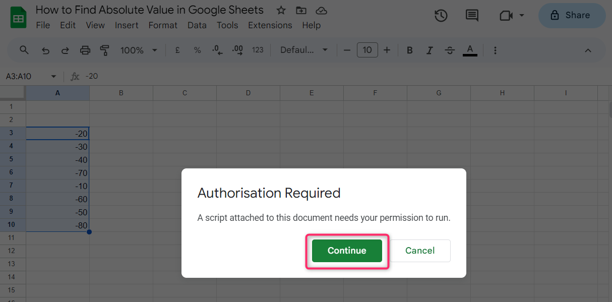
Step 7: The first time when you apply the script, you will be asked for the authentication. Click on Continue to give permission to run the script by following the instructions:

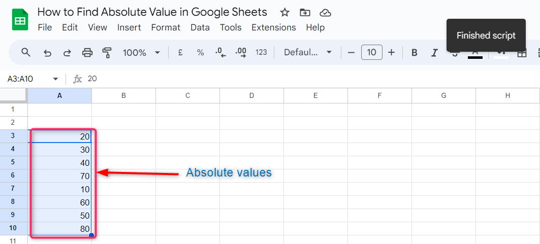
Step 8: You will get the absolute values of all the entries in the selected data in the same column where they were placed before:
Method 4: Find Absolute Values Using Power Tools Feature In Google Sheets
Power Tools in Google Sheets is the set of more than 30 features that provide the solutions for most common and complicated tasks. By using the power tools feature in Google Sheets, we can remove the negative signs from the less than zero value in large data collectively to get their absolute values without hurting the positive values.
Follow the following Steps to learn how to use the power tool feature in Google Sheets to find the absolute values by taking the previous example.
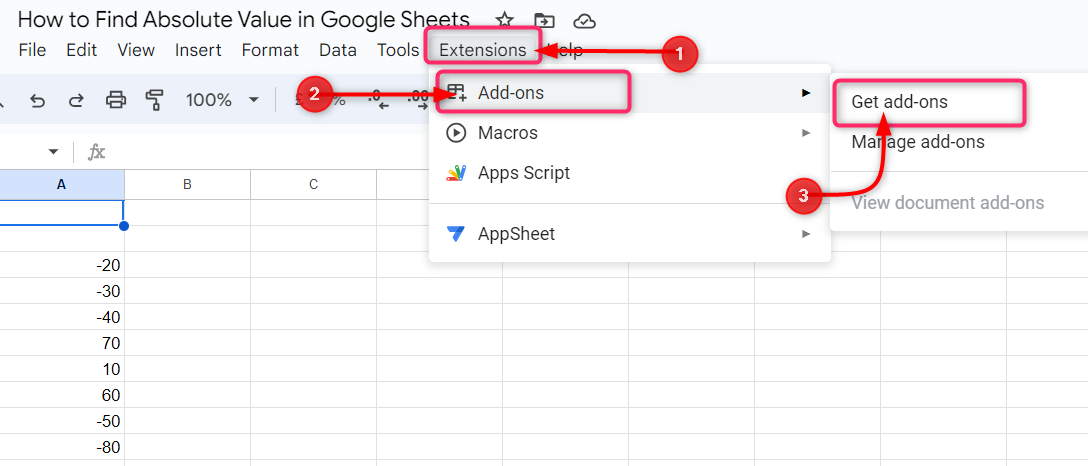
Step 1: Click on Extensions from the taskbar, then click on Add-ons from the dropdown menu. In the Add-ons’ dropdown menu, click on Get add-ons:
Step 2: Search for Power Tools in the Google Workspace Marketplace web page and install the Power Tools app. This will require authentications to grand access to your Google account. Foolow the instructions and allow the app to get access to your Google account:

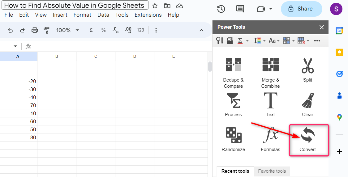
Step 3: After completing the installation of the Power Tools, it will appear on the right side in Google Sheets. Click on the Convert from the Power Tools menu:
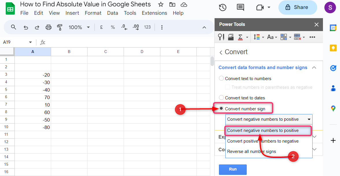
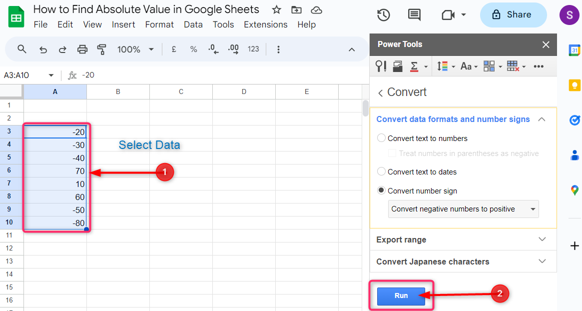
Step 4: Select Convert number sign and click choose Convert negative numbers to positive in the dropdown menu. This action will only convert the signs of the negative number and keep the positive number remain unchanged:
Step 5: Now select the data from which you want to find the absolute values, then click on Run in the Power Tools section:
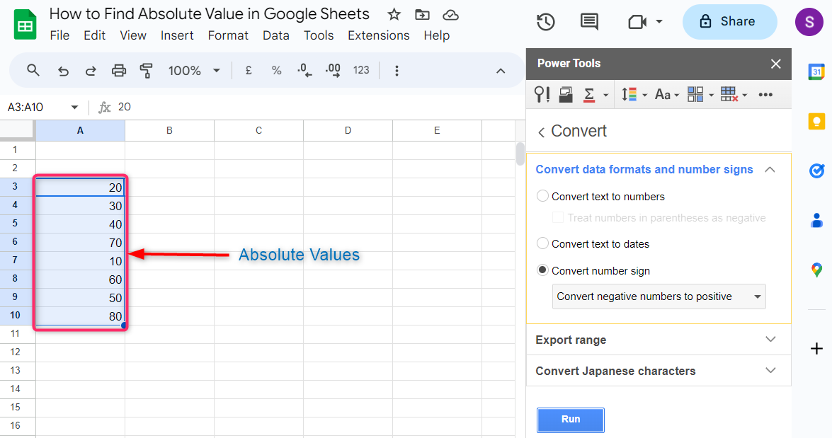
Step 6: You will get the absolute values in return after removing the negative signs from the less than zero values:
Conclusion
Dealing with large data, to find absolute values, it is hard to convert negative signs of less than zero values by ignoring the positive values. Google Sheets has useful functions and features to do this job. Click on an empty cell and apply the ABS() function with reference to the first cell of the data, then copy the applied function and paste it to more empty cells equal to the number of cells and columns in the original data. The IF() function also works as the ABS() does. Click on extensions and go to Add-ons. Download the power tools app from Add-ons and run its convert feature as mentioned above to find the absolute values.