Machine Learning uses the models to get insights or hidden patterns from the given dataset based on historical facts. ML uses supervised and unsupervised learning techniques to get the predictions after training. Supervised learning means that the dataset has the output field available in the dataset and the unsupervised learning doesn’t have the output values. The loss functions in machine learning are used to optimize the performance of the artificial intelligence models.
Quick Outline
This guide explains the following sections:
- What is NLL Loss
- How to Calculate NLL Loss of DL Model in PyTorch
What is NLL Loss
The Negative Log Likelihood (NLL) is used to evaluate the performance of the model with the unbalanced training data. It takes the probabilities of the correct predictions but it does not only work with the correct predictions made by the model. With that, the model is appreciated for high probabilities of the correct prediction and punished for low probabilities of the correct prediction. It means that the NLL loss gives more value to the confidence of the method while predicting the correct values.
The mathematical representation of the NLL loss is mentioned below:

Here:
x: specifies the input values in the data
y: suggests the target values
T: predicted values related to positive classes
w: contains the weights of the relation between different layers of the neural network
N: tells the size of the batch
The NLL loss function normalizes the actual values within the range from 0 to 1 using the softmax() function in PyTorch. Taking the logarithm of these values will generally provide a negative value and then it applies the negative sign to the complete value.
How to Calculate NLL Loss of DL Model in PyTorch
Deep Learning models use neural networks to teach the machine using multiple iterations of going over the dataset. Usually, deep learning models take more time and computational power to learn than the machine learning model but they produce better results to compensate for that loss. The loss functions provide us with a better view of the model’s performance throughout these iterations. The following steps implement the process by building the model and producing loss values for all the training batches:
Note: The code used in this guide which is written in Python programming language is available here:
Step 1: Access Python Notebook
The first step here is to create a new notebook to write the Python code and it can be done using Jupyter, VS Code, Google Colab, etc. This guide builds the project in the Google Colab notebook which can be accessed from the official website:

Step 2: Install Modules
In the notebook, start writing the code to install the torch module for accessing its libraries and dependencies. The pip command which is the package manager for the Python language can be used to install the module:
pip install torchStep 3: Import Libraries
Now, import the libraries that are required to perform all the steps to build and train the model with the loss values:
import os
import torch
from torch import nn
from torchvision.datasets import MNIST
from torch.utils.data import DataLoader
from torchvision import transforms- The os library is used to access the operating system to provide the computational power that the model requires.
- Torch is the main library here to give access to the neural network models using the nn dependency and DataLoaders for the data as well.
- The MNIST contains the dataset that has multiple classes in the output field making it a good fit for the application of the NLL loss method in PyTorch.
- Torchvision library is used to import the transformers for converting the large data into smaller batches for better management.
Step 4: Configuring MLP Neural Networks
After getting the required libraries, build the Multilayer Perceptron neural network model that works better for multi-class data. The normal neural network contains three layers with input, hidden, and output layers to train the model. MLP uses a multilayered approach by adding another layer before the output layer to perform the activation function on the output of the hidden layers. After getting through the additional layer, the output layer receives the data to give the predictions as the following code suggests:
class MLP(nn.Module):
  '''
    MLP or Multilayer Perceptron Model
  '''
  def __init__(self):
    super().__init__()
    self.layers = nn.Sequential(
      nn.Flatten(),
      nn.Linear(28 * 28 * 1, 64),
      nn.ReLU(),
      nn.Linear(64, 32),
      nn.ReLU(),
      nn.Linear(32, 10),
      nn.LogSoftmax(dim = 1)
    )

  def forward(self, x):
    '''Forward pass'''
return self.layers(x)- The code builds the MLP class with the neural network modules imported from the torch library
- Define the constructor to build the structure of neural networks with the Sequential() method to be stored in the layers variable.
- In the sequential model, each layer is attached to its previous and next layer in a sequence starting with the input and going to the output layer.
- Each process in this approach has to follow the previous layers as it can only work if the previous layer has completed its work.
- The above code builds three layers with different numbers of neurons and the dimensions of the input and output features.
- Add the LogSoftmax() method with the dimension of the additional layer to apply the normalization on the dataset while training.
- Define the forward() method to make the model using the feed-forward technique using the layers variable from the constructor.
- The feed-forward approach means that the model only goes in the forward direction to find the predictions.
- On the other hand, backpropagation means that the model goes back to adjust its weights and bias to minimize the loss value.
Step 5: Getting the MNIST Dataset
Once the model is built, it is time to feed the dataset to get insights or hidden patterns from the data:
if __name__ == '__main__':
  torch.manual_seed(42)
  dataset = MNIST(os.getcwd(), download=True, transform=transforms.ToTensor())
  trainloader = torch.utils.data.DataLoader(dataset, batch_size=10, shuffle=True, num_workers=1)
mlp = MLP()- The MNIST() method can be used to get the dataset and then the DataLoader() with its arguments can be used to load the data.
- The arguments of the MNIST() method use the operating system to get the data and keep the download value as true to get the data.
- The transformer argument uses the To.Tensor() method to convert the dataset to the tensors in the PyTorch.
- The arguments of the DataLoader() method are used to load the structure of the data according to the requirement.
- Call the MLP() class with the neural network structure in the main to integrate the dataset with the deep learning model:
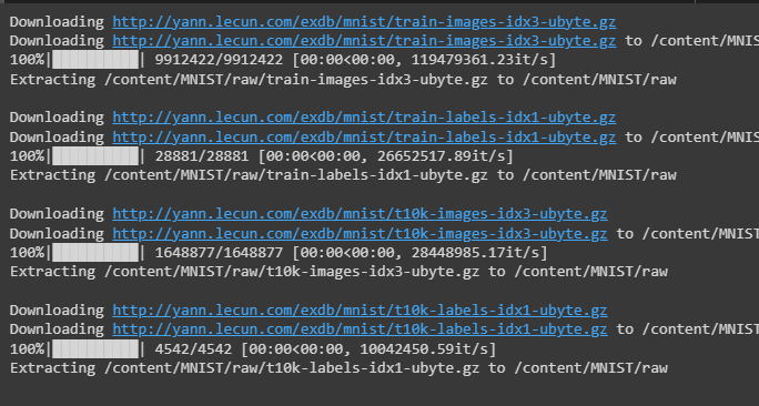
The following screenshot displays that the dataset is being downloaded from the MNIST library:

Step 6: Calling the NLLLoss() Method
After getting the dataset in the desired format, it is important to call the desired lossfuntion according to the problem that the model is trying to solve:
loss_function = nn.NLLLoss()
optimizer = torch.optim.Adam(mlp.parameters(), lr=1e-4)- Call the NLLLoss() method with the nn dependency and store it in the loss_function variable.
- Use the Adam() optimizer from the optim dependency of the torch library with the parameters() method for the MLP method and the learning rate of the model.
Step 7: Training the Deep Learning Model
Now that the model is ready with the data and loss function, simply train the deep learning model with multiple iterations:
for epoch in range(0, 5):
    print(f'Starting epoch {epoch+1}')
    current_loss = 0

    for i, data in enumerate(trainloader, 0):
      inputs, targets = data
      optimizer.zero_grad()
      outputs = mlp(inputs)
      loss = loss_function(outputs, targets)
      loss.backward()
      optimizer.step()
      current_loss += loss.item()
      if i % 500 == 499:
          print('Loss after mini-batch %5d: %.3f' %
                (i + 1, current_loss / 500))
          current_loss = 0

print('Training process has finished')- Use the for loop to control the number of iterations for the model by providing the range for the epoch variable.
- Apply the nested for loop to train the model with the data using the trainloader variable as the range of the loop.
- Give the data to input and target variables as the input is provided by the user and the output values are extracted from the predictions.
- Once the input and output values are extracted, apply the loss() method to check the performance of the model with each inner loop.
- After getting the loss value, apply the backpropagation to minimize the loss value and then apply the optimizer with the step() method.
- The optimizer is used to adjust the values of the bias and weights while backpropagation to optimize the model’s performance.
- After that, set the conditional statement to get the loss value for each iteration in the inner loop using the current_loss variable.
- Finally, print the end message at the end of all the iterations or epochs which means that the model is trained:
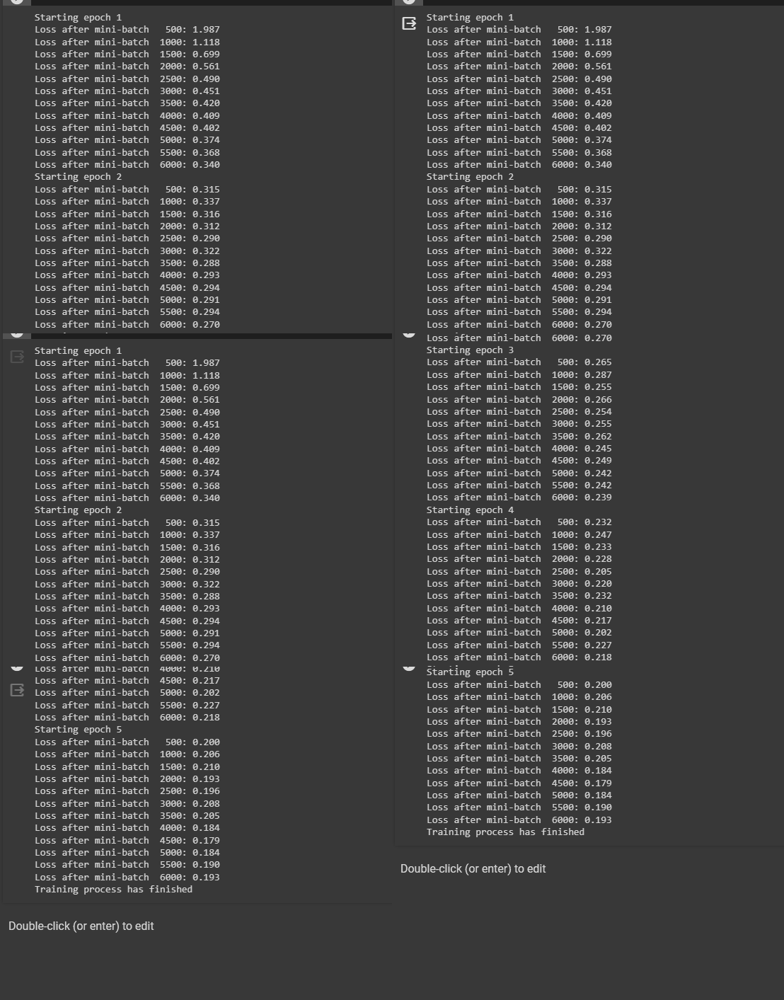
The following screenshot displays that the loss value is going down with each batch and the epoch in general. The loss value for the first batch is 1.987 which is not a very good performance but at the end of the training, the loss value becomes 0.193. The loop with 5 iterations makes the model more efficient and optimized with minimum loss value:

That’s all about the process of calculating the Negative Log Likelihood Loss on the trained deep learning model in PyTorch.
Conclusion
To calculate the Negative Log Likelihood loss of the deep learning model, build the deep learning model using the neural network structure. After that, download the MNIST dataset that has multiple classes for the output field. The NLL loss value is preferably used to solve the multi-class classification using a neural network algorithm like the MLP model. The model is trained on multiple iterations with mini-batches to keep track of the loss values for each iteration.