Machines are trained in Machine Learning or Artificial Intelligence to make predictions using the input data given by the user. Machines are not always accurate as there is always room for error and the loss functions can be used for evaluation. PyTorch framework is used to build neural network models with built-in loss functions to keep an eye on their performance.
PyTorch offers multiple loss methods to find the error value using different aspects of the model. The user has to look at the structure of the model and evaluate it accordingly. The user can extract the correct evaluation method by understanding the problem in the model by analyzing the dataset. Understand the evaluation method and apply it to the model to minimize the error in the performance.
Quick Outline
This guide explains the following sections:
- What is L1/MAE Loss
- How to Calculate MAE/L1 Loss of DL Model in PyTorch
What is L1/MAE Loss
The Mean Absolute Error or MAE also called the L1 loss value takes the difference between the predicted values from the actual ones. After finding the difference, the function takes the absolute of the difference to make all the values positive. Now, it adds the absolute difference values and then divides them by the total size of the dataset. Without the absolute difference, the positive and negative errors cancel each other and the loss value will become significantly low.
The mathematical representation for the Mean Absolute Error or L1 is as follows:

Here:
MAE: Mean Absolute Error
P: Predicted values
A: Actual values from data
N: Total size of the data
How to Calculate MAE/L1 Loss of DL Model in PyTorch
Finding the L1 loss of the deep learning model in pytorch requires the installation of the torch module from Python’s package manager. After that, build the structure of the neural network with its neurons and train the model using the input dataset provided by the user. Configure the loss value to optimize the performance of the model and graphical representations can be used to check the improvements. To learn the process of calculating the L1 loss in PyTorch, simply go through the following steps:
Note: The Python notebook with the code used in this guide is attached here
Step 1: Accessing Python Notebook
The first step is creating a new project in a Python notebook like Jupyter, Google Colab, etc. This guide uses the Google Colab Notebook which can be accessed from the official website:

Step 2: Installing Modules
Once the notebook is created, install the torch module using the pip (Python package manager) command to access the libraries stored in it:
pip install torchStep 3: Importing torch Libraries
Building the deep learning model and calculating the L1 loss values in PyTorch require different functions from the torch module. To use these functions, simply import the required libraries like nn for neural network and pyplot for plotting graphs using the following code:
import torch
from torch import nn
import matplotlib.pyplot as plt
Step 4: Building Dataset With Model’s Parameters
Now, build the dataset for training the neural network with the external parameters like weight and bias required to train the model:
weight = 0.7
bias = 0.3
start = 0
end = 1
step = 0.02
X = torch.arange(start, end, step).unsqueeze(dim=1)
y = weight * X + bias

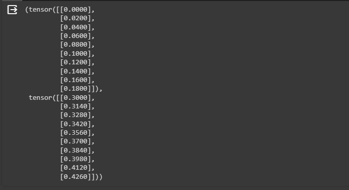
X[:10], y[:10]- The neural network model uses neurons spread across multiple layers as the first layer gets the actual input and the last layer produces the outputs.
- The neuron can not be connected with the neuron of the same layer, it can only be connected to the neurons of the next layer.
- The pathway that connects the neuron from the first layer to the second layer contains the weight parameter and the bias is the external input to normalize the predictions.
- The weight parameter is used with the input values in the activation function to produce the output value which is then provided to the next layer.
- Build the dataset using the arange() method in X variable with the values starting from 0 and ending when values become 1 with the steps between each value.
- Create another variable called y for producing outputs and it takes values using the weight, bias, and X variables.
- Print the first 10 values of the tensors of X and y tensors as displayed in the screenshot below:
Step 5: Splitting Data
After generating the dataset, simply split the actual values into training and testing datasets using the 80-20 split. The 80-20 split means that 80% of the values would be considered as training data and the 20% will be used as the testing data:
train_split = int(0.8 * len(X))
X_train, y_train = X[:train_split], y[:train_split]
X_test, y_test = X[train_split:], y[train_split:]

len(X_train), len(y_train), len(X_test), len(y_test)- Train the model using the training data which is 80% of the actual data and then test the model on the rest of the 20% data.
- The data is split into training and testing data to check the performance of the model on the unseen but similar dataset.
- Print the length of testing and training sets for both X and y variables:

Step 6: Plotting the Actual Data
Define the plot_prediction() method using the training, testing, and prediction values to display the graph on the screen:
def plot_predictions(train_data=X_train,
                    train_labels=y_train,
                    test_data=X_test,
                    test_labels=y_test,
                    predictions=None):

  plt.figure(figsize=(10, 7))
  plt.scatter(train_data, train_labels, c="b", s=4, label="Training data")
  plt.scatter(test_data, test_labels, c="g", s=4, label="Testing data")

  if predictions is not None:
    plt.scatter(test_data, predictions, c="r", s=4, label="Predictions")
plt.legend(prop={"size": 14});- Use the train_data, train_labels, test_data, test_labels, and predictions arguments to define the plot_predictions() method.
- The figure() method is used to set the dimensions for the graph with the size of the figure using the figsize variable.
- Use the scatter() method to plot the training and testing data using the dots of blue and green colors respectively.
- Use the conditional statement to display the prediction data if the prediction variable has some values.
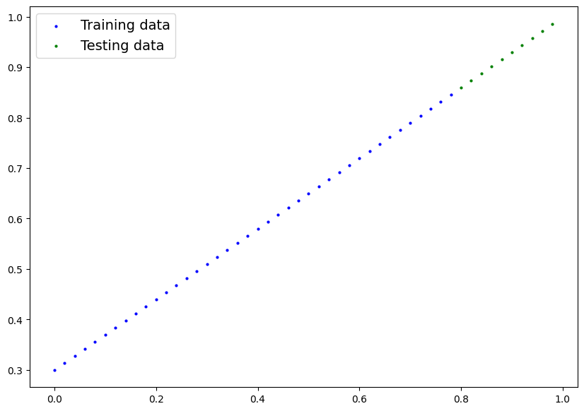
Plot the graph by calling the plot_predictions() method defined in the previous code block:
plot_predictions()The following screenshot displays the training and testing data with dots starting from 0 and ending at 1 as the parameters suggested. 80 percent of the data is colored blue referring to the training data and the green dots for the testing data:
Step 7: Building the Model
After that, simply build the LinearRegressionModel using the neural network module from the torch library with layers configuration. Configure the different layers of the neural network by configuring the parameters like neurons for the weight and bias of each layer. Apply the feed-forward approach to build the activation function to calculate the output value using the weight, bias, and input value:
class LinearRegressionModel(nn.Module):
    def __init__(self):
        super().__init__()
        self.weights = nn.Parameter(torch.randn(1, dtype=torch.float), requires_grad=True)
        self.bias = nn.Parameter(torch.randn(1, dtype=torch.float), requires_grad=True)

    def forward(self, x: torch.Tensor) -> torch.Tensor:
        return self.weights * x + self.bias
Normalize the data using the manual_seed() method and then store the LinearRegressionModel() in the model_0 variable:
torch.manual_seed(42)

model_0 = LinearRegressionModel()
list(model_0.parameters())
Print the stored type of the model in the torch dictionary using the following code:
model_0.state_dict()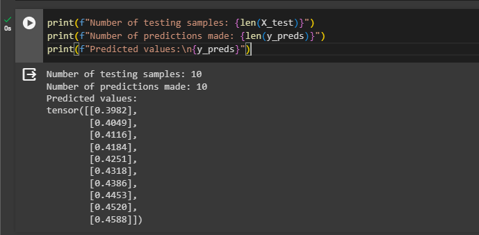
Step 8: Testing the Model
Now, test the model using the model_0 variable and store the values in the y_preds variable using the inference_mode() method from torch:
with torch.inference_mode():
    y_preds = model_0(X_test)
Print the lengths of the testing and prediction values from the overall dataset before printing the predicted values:
print(f"Number of testing samples: {len(X_test)}")
print(f"Number of predictions made: {len(y_preds)}")
print(f"Predicted values:\n{y_preds}")
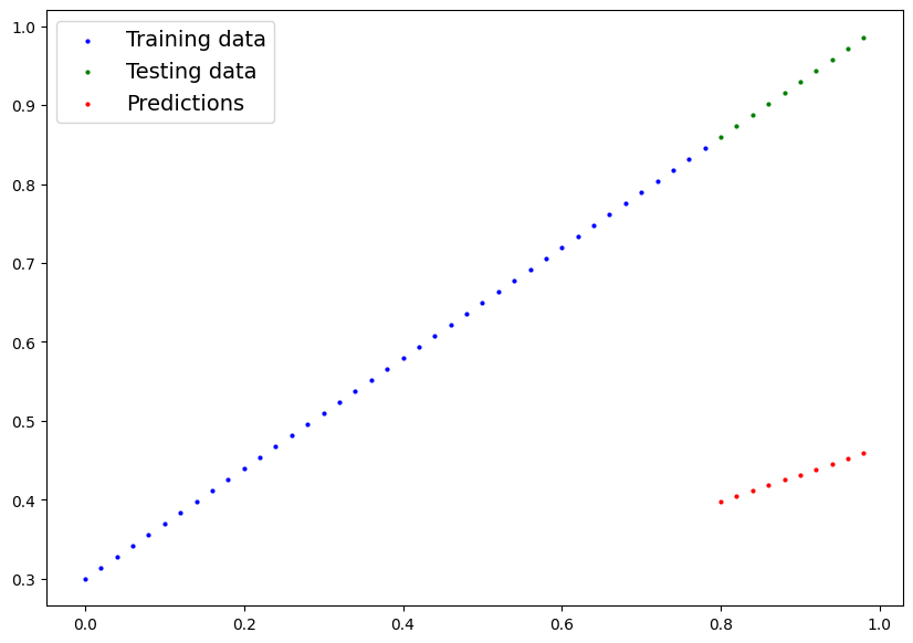
Plot the predicted values with the training and testing values using the scatter graph:
plot_predictions(predictions=y_preds)The following graph displays the prediction from a feed-forward model that only uses external values to generate predictions. Its predictions are not very accurate and to optimize its performance, we need to apply backpropagation while training the model:
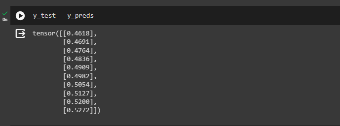
The user can find the loss values manually by subtracting the test values from the predicted values as mentioned below:
y_test - y_predsThe difference values are very high and the model has not predicted accurately as displayed below:
Step 9: Configuring L1 Loss Value
Here, find the loss using the proper method called the L1Loss() method provided by the torch library and store it in the loss_fn variable. Optimize the model with different arguments like params and learning rate:
loss_fn = nn.L1Loss()
optimizer = torch.optim.SGD(params=model_0.parameters(), lr=0.01)
Step 10: Training the Model
Use the loss function to get the optimized predictions using multiple iterations that allow the model to learn the insights from the dataset:
torch.manual_seed(42)

epochs = 100
train_loss_values = []
test_loss_values = []
epoch_count = []

for epoch in range(epochs):
    model_0.train()
    y_pred = model_0(X_train)
    loss = loss_fn(y_pred, y_train)
    optimizer.zero_grad()
    loss.backward()
    optimizer.step()
    model_0.eval()

    with torch.inference_mode():
      test_pred = model_0(X_test)
      test_loss = loss_fn(test_pred, y_test.type(torch.float))

      if epoch % 10 == 0:
            epoch_count.append(epoch)
            train_loss_values.append(loss.detach().numpy())
            test_loss_values.append(test_loss.detach().numpy())
print(f"Epoch: {epoch} | MAE Train Loss: {loss} | MAE Test Loss: {test_loss} ")- Set the epoch size to get 100 iterations for the model using the train, test, and epoch count.
- After setting the values, simply use the for loop to store the prediction values in the y_pred variable.
- Apply all the components like loss, optimizer, backward, and model to train the model to use the L1 loss and regression model.
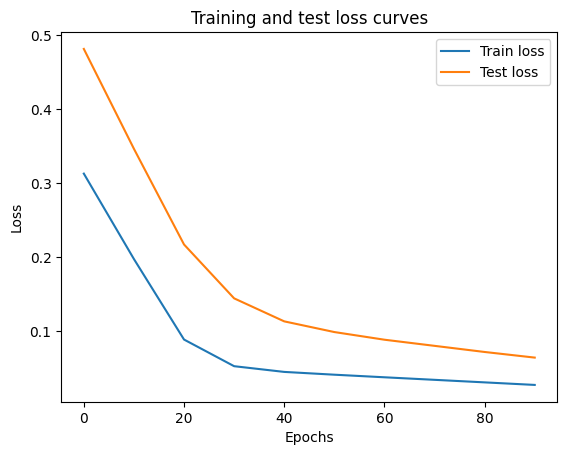
- Print the training and testing loss values once after 10 iterations. The loss value goes down after each iteration as displayed in the screenshot below:

Step 11: Plotting the Loss Values
Plot the loss values for both training and testing data across each epoch using the following code:
plt.plot(epoch_count, train_loss_values, label="Train loss")
plt.plot(epoch_count, test_loss_values, label="Test loss")
plt.title("Training and test loss curves")
plt.ylabel("Loss")
plt.xlabel("Epochs")
plt.legend();- Use the epoch_count and train_loss_values with the train and test loss labels in the plot() method.
- Displays the loss values across all the epochs as displayed in the following screenshot:
Step 12: Comparing Testing and Prediction Values
Call the eval() method to perform the evaluation of the model using the model_0 variable and store the values in the y_preds variables:
model_0.eval()
with torch.inference_mode():
  y_preds = model_0(X_test)
y_preds
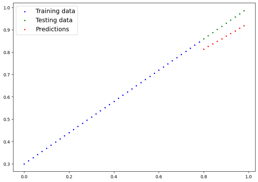
Plot the values stored in the y_preds with the training and testing data to compare the testing values with predictions:
plot_predictions(predictions=y_preds)Using the Mean Absolute Error, the model has evaluated itself throughout 100 iterations and predicted way better than the last predictions. So the model has been optimized using the loss values generated across each iteration using the epoch argument:
That’s all about calculating the L1 loss value from the deep learning model in PyTorch.
Conclusion
To calculate the Mean Absolute Error or L1 loss values for the trained deep learning model, build a model and optimize its performance using the loss values. The model is trained using multiple iterations in batches to keep the loss value minimum. Graphical representation can be used to check the evolution of the model across each iteration and confirm the model’s growth.