Classification is the supervised learning method in the Artificial Intelligence domain where the model is trained using the labeled data. It means that the actual data contains the output data from the past and the model has to predict the future using it. The loss functions are used to optimize the performance of the AI model like using the Hinge loss methods using the PyTorch. Hinge loss generally performs well in optimizing the models that are solving the classification problems in machine learning.
Quick Outline
This guide explains the following sections:
- What is Hinge Loss
- How to Calculate Hinge Loss in PyTorch
- Method 1: Calculate Hinge Loss for Sequential Model
- Method 2: Calculate Hinge Loss Using HingeEmbeddingLoss() Function
- Method 3: Calculate Loss Using HingeLoss() Function
- Method 4: Calculate Hinge Loss Using Functional Multi-Class
- Method 5: Calculate Hinge Loss Using BinaryHingeLoss() Function
- Conclusion
What is Hinge Loss
The Hinge Loss is used to measure the performance of the model by separating the correct and wrong predictions within two classes. In classification, the Hinge Loss is mainly used in the Support Vector Machine or SVM algorithm to get the maximum margin of the classification. The mathematical representation of the hinge loss is mentioned below:
y: Predicted value
t: Input value
The hinge loss classifies the predicted data into correct predictions and wrong predictions. If the “t.y”? 1 then it means that all the correct values are in this section and the hinge loss value becomes 0. For “t.y” < 1 means that the class contains the incorrect predictions and the hinge loss value starts to increase.
How to Calculate Hinge Loss in PyTorch
The PyTorch environment offers multiple functions like HingeLoss(), HingeEmbeddingLoss(), and BinaryHingeLoss() to calculate the hinge loss values. These methods can be used to enhance the performance of the neural network models by applying training iteration. To learn the process of implementing these methods and finding the loss value, simply go through the following methods:
Note: The Python code to calculate the hinge loss is available here
Method 1: Calculate Hinge Loss for Sequential Model
The sequential model takes one input and produces one output with all the intermediate steps following the previous one in a sequence. It implements one step at a time to generate the prediction according to the sample dataset and plots their values on the screen. To implement the model and evaluate its loss values, simply go through the following steps:
Step 1: Access Python Notebook
To write the Python code, open a notebook like VSCode, Jupyter, or Google Colab to create a fresh project. This guide uses the Google Colab notebook which can be accessed from the official website:

Step 2: Install Modules
Install the torchmetrics module containing the metrics for machine learning distributions to build the deep learning models in the torch framework. Use the pip command to install the torchmetrics dependencies to use the hinge methods provided by torch:
pip install torchmetrics
Step 3: Importing Libraries
Now, import the required libraries for building the dataset and train the deep learning model on that. These libraries are also required to evaluate the performance and display it on the screen:
from keras.optimizers import SGDfrom sklearn.datasets import make_circlesfrom matplotlib import pyplot
from keras.models import Sequentialfrom numpy import where
from keras.layers import Dense
Step 4: Building a Model
Start the process by building the dataset for the model using the make_circles() method with multiple arguments like samples, noise, and randomness. The X dataset contains the input values and the y variable will be used to store the predicted values provided by the model after testing:
X, y = make_circles(n_samples=1000, noise=0.1, random_state=1)
y[where(y == 0)] = -1
Now, train the model using the portion of the dataset so the model can find the hidden patterns from the data and then the rest will be used to test the model:
n_train = 500
trainX, testX = X[:n_train, :], X[n_train:, :]
trainy, testy = y[:n_train], y[n_train:]
Call the sequential() method to initialize the model value and store its values in the variable:
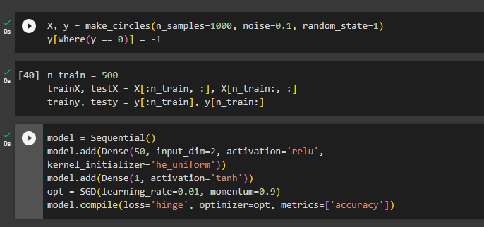
model = Sequential()
model.add(Dense(50, input_dim=2, activation='relu',
kernel_initializer='he_uniform'))
model.add(Dense(1, activation='tanh'))
opt = SGD(learning_rate=0.01, momentum=0.9)
model.compile(loss='hinge', optimizer=opt, metrics=['accuracy'])
The above code:
- Call the model variable to add the denser with the number of neurons which is 50 here, 2 dimensions, and the rectified linear unit(relu) activation functions.
- After that, add another layer with a single neuron and the tanh activation function to get better performance for the multi-layer neural network.
- Design the opt variable to call the Stochastic Gradient Descent or SGD() method with the learning rate of 0.01 and the 0.9 momentum
- In the end, compile the model to find the value of the “hinge loss”, optimizer, and accuracy:

Step 5: Training the Model
After building the model, initialize the history variable with the model.fit() method using the training sets of the input and predicted data. The test data from both sets are used to validate the performance of the model during 200 epochs as the following code suggests:
history = model.fit(trainX, trainy, validation_data=(testX, testy), epochs=200, verbose=0)Use the evaluate() method with the model variable to get the validation values of the model from the training and testing data:
_, train_acc = model.evaluate(trainX, trainy, verbose=0)#Model evaluation using the training variables
_, test_acc = model.evaluate(testX, testy, verbose=0)#Model evaluation using the testing variables
print('Train: %.3f, Test: %.3f' % (train_acc, test_acc))
Step 6: Plotting the Values
Once the values are calculated, simply plot the values of the loss for training and testing data on the graph using the following code:
pyplot.subplot(211)
pyplot.title('Loss')
pyplot.plot(history.history['loss'], label='train')
pyplot.plot(history.history['val_loss'], label='test')
pyplot.legend()
The following screenshot displays the loss values of the training and testing during the 200 epochs. The start was a bit off but as the epochs started to increase, the loss value kept decreasing. The prime objective is to minimize the loss value and there comes a time when the line becomes horizontal without changing its direction. At that moment the model is completely optimized and there is no further chance of improvement left:

The following code builds the visualization using a line graph for different accuracy points throughout the 200 epochs. The graph displays two lines referring to the accuracy of the model for the training and testing data sets:
pyplot.subplot(212)
pyplot.title('Accuracy')
pyplot.plot(history.history['accuracy'], label='train')
pyplot.plot(history.history['val_accuracy'], label='test')
pyplot.legend()
pyplot.show()
The following screenshot displays the graph for the accuracy of the model for training and testing data set. The visualization tells us that the accuracy increases with the epochs going above 35% starting from 0 which can be improved with a more versatile dataset:

Method 2: Calculate Hinge Loss Using HingeEmbeddingLoss() Function
The torch also allows the use of the HingeEmbeddingLoss() method to find the hinge loss value in Python programming language. The Embedding loss in PyTorch is often used for binary classification with simplified values and storing large data in a database or tensors in PyTorch. To implement the HingeEmbeddingLoss() method, simply go through the following examples:
Example 1: Using HingeEmbeddingLoss With Neural Network
The following code implements the HingeEmbeddingLoss() method to find the difference between the original and predicted values:
input = torch.randn(3, 5, requires_grad=True)
target = torch.randn(3, 5)

hinge_loss = torch.nn.HingeEmbeddingLoss()
output = hinge_loss(input, target)
output.backward()

print('output: ', output)
The code:
- Uses the HingeEmbeddingLoss() method which is used to perform binary classification in hinge loss.
- It also creates input and target tensors with multi-dimensional structures and calls the HingeEmbeddingLoss() with the neural network dependency.
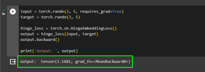
- After that, apply the backpropagation to the loss function using the backward() method on the output variable and print the loss value on the screen:
Example 2: Using HingeEmbeddingLoss With MLP Model
The following code uses the Multilayer Perceptron or MLP model which is an artificial neural network model with connected neurons. The connected neurons mean that each neuron is connected to every neuron of the preceding layer and the data is transferred through multiple sources:
from torchvision.datasets import FakeDatafrom torchvision import transformsimport osfrom torch.utils.data import DataLoader
from torch import nn

class MLP(nn.Module):
  '''
    Multilayer Perceptron Model
  '''
  def __init__(self):
    super().__init__()
    self.layers = nn.Sequential(
      nn.Flatten(),
      nn.Linear(28 * 28 * 3, 64),
      nn.ReLU(),
      nn.Linear(64, 32),
      nn.ReLU(),
      nn.Linear(32, 1),
      nn.Tanh()
    )

  def forward(self, x):
    '''Forward pass between the layers'''
    return self.layers(x)

if __name__ == '__main__':
  torch.manual_seed(42)

  dataset = FakeData(size=15000, image_size=(3, 28, 28), num_classes=2, transform=transforms.ToTensor())
  trainloader = torch.utils.data.DataLoader(dataset, batch_size=64, shuffle=True, num_workers = 4, pin_memory = True)
  mlp = MLP()

  # Using HingeEmbeddingLoss()
  loss_function = nn.HingeEmbeddingLoss()
  optimizer = torch.optim.Adam(mlp.parameters(), lr=1e-4)

  for epoch in range(0, 5):
    print(f'Starting an Iteration {epoch+1}\n')
    current_loss = 0

    for i, data in enumerate(trainloader, 0):
      inputs, targets = data
      targets[targets == 0] = -1
      targets = targets \
                  .type(torch.FloatTensor) \
                  .reshape((targets.shape[0], 1))

      optimizer.zero_grad()
      outputs = mlp(inputs)
      loss = loss_function(outputs, targets)
      loss.backward()
      optimizer.step()
      current_loss += loss.item()

      if i % 10 == 0:
          print('Loss after mini-batch %5d: %.3f' %
                (i + 1, current_loss / 500))
          current_loss = 0.0

  print('Training process has finished')
The above code:
- Imports the required libraries like os, nn, FakeData, transforms, and DataLoader to build the MLP model.
- The os is used to interact with the operating system and nn is used to call the neural network models offered by the torch library.
- The other libraries are for getting and managing data for the model to evaluate the loss value of the model.
- The above code simply uses the class MLP with the neural network model that consists of three layers with connected neurons.
- The first layer produces 64 outputs using the Flatten() method and all these outputs act as the inputs for the next layer.
- The next layer takes the 64 inputs and produces 32 outputs for the final layer and the final input evaluates all of them to produce a single output.
- The model uses the feed-forward techniques to give data for the first layer and its output goes as input for the first layer to produce the loss value.
- The input value is given to the model from the FakeData library offered by the torch library and the HingeEmbeddingLoss() method gets the loss value.
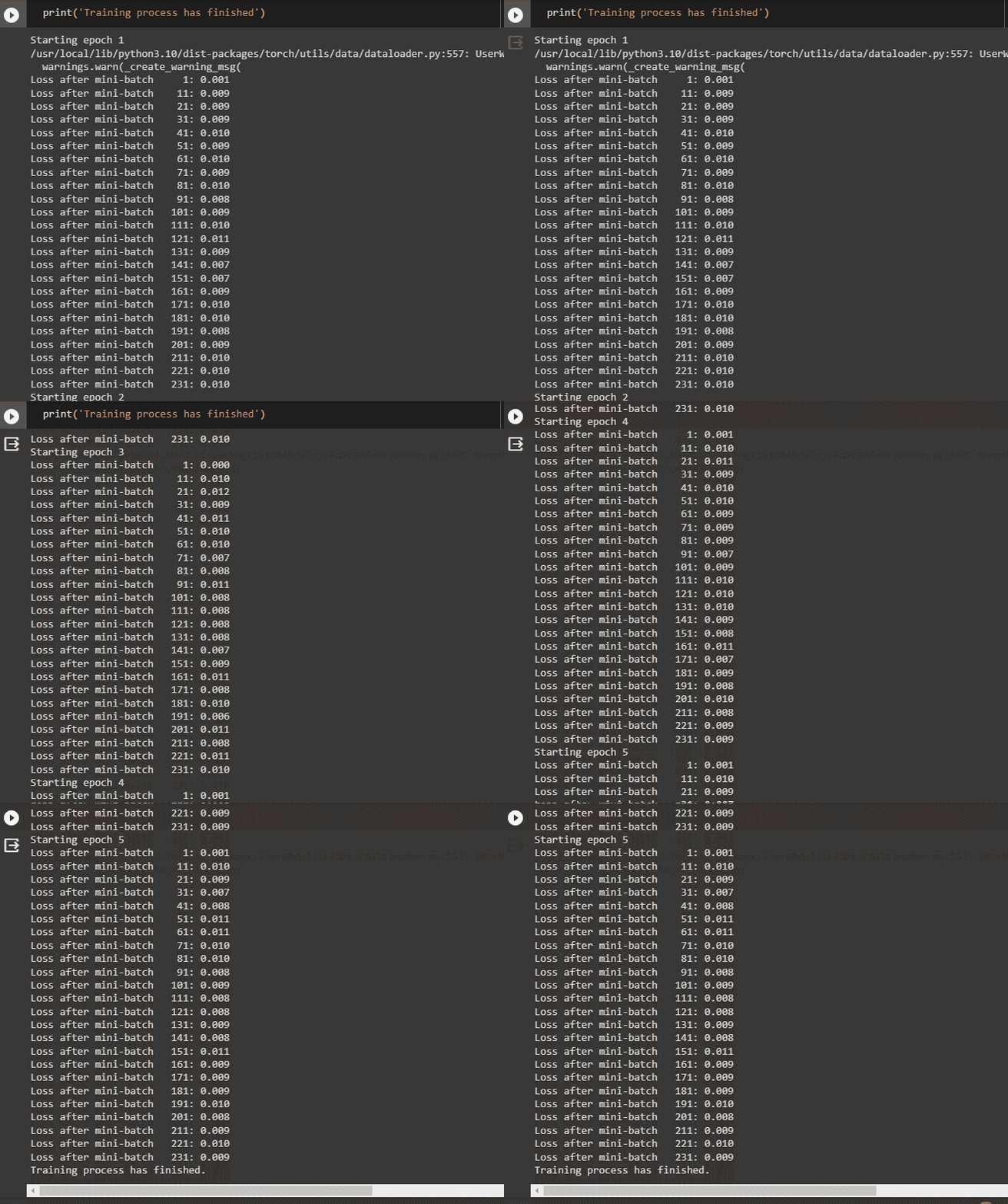
- The neural network model is optimized using the Adam() method while running each of the 5 epochs with 10 mini-baches:
- The following screenshot displays the loss value for each minibatch for all 5 epochs before printing the finished message:
Method 3: Calculate Loss Using HingeLoss() Function
This method uses the HingeLoss() method offered by the torch library to calculate the loss values between the input and predicted data. This loss value can be used to evaluate the performance of the model as it explains how many wrong predictions are made by the model. It also takes the intensity of the correct and wrong predictions into account to make a more accurate evaluation of the model. Start the process of implementing the HingeLoss() method using the following steps:
Step 1: Import Libraries
Import the torch library to use its functions and calculate the hinge loss value in the Python language:
import torchPrint the installed version of the torch framework to confirm that it is ready for use:
print(torch.__version__)
Step 2: Calculate Hinge Loss With Binary Task
Once the torch environment is set, simply start implementing the code by importing the tensor and HingeLoss libraries from the installed framework. The tensor library is used to create the datasets in the torch and HingeLoss is the function to calculate the value of the loss using the following code:
from torch import tensor
from torchmetrics import HingeLoss

target = tensor([0, 1, 1])
preds = tensor([0.5, 0.7, 0.1])
hinge = HingeLoss(task="binary")
hinge(preds, target)
The above code:
- Creates two tensors as the first one contains the actual values and the second one contains the predicted values from the model.
- Defines the hinge variable to call the HingeLoss() method with the binary task to evaluate the true or false predictions and find the loss value.
- The following screenshot displays the hinge loss value evaluated using the target and predicted tensors:

Method 4: Calculate Hinge Loss Using Functional Multi-Class
The multi-class tasks mean that target values have more than one class of prediction to evaluate the performance of the model. The multiclass_hinge_loss can be imported from the functional dependency of the torch to solve the classification problems in Machine Learning:
from torch import tensor
from torchmetrics.functional.classification import multiclass_hinge_loss
preds = tensor([[0.25, 0.20, 0.55],
                [0.55, 0.05, 0.40],
                [0.10, 0.30, 0.60],
                [0.90, 0.05, 0.05]])
target = tensor([0, 1, 2, 0])
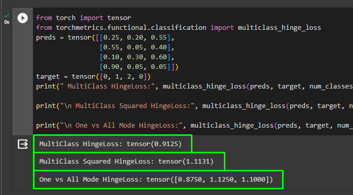
print(" MultiClass HingeLoss:", multiclass_hinge_loss(preds, target, num_classes=3))

print("\n MultiClass Squared HingeLoss:", multiclass_hinge_loss(preds, target, num_classes=3, squared=True))

print("\n One vs All Mode HingeLoss:", multiclass_hinge_loss(preds, target, num_classes=3, multiclass_mode='one-vs-all'))
The above code:
- Creates tensors and applies the multiclass_hinge_loss() method with the number of classes and tensors as the argument.
- The input dataset is compared with the predicted values to classify them between the given number of classes and then finds the loss value.
- The squared hinge loss simply takes the square of the loss value to make the numerical values more readable.
- In squared hinge loss, the input values must belong to the {1, -1} set of numbers so it also provides the smoothing effect to the values.
- The multiclass_mode is the argument while calling the multiclass_hinge_loss() method to map the target tensor with the prediction one.
- The prediction tensor contains multiple classes and the model contains the one-vs-all value, meaning each prediction class matches the original value.
- In the end, simply print the loss values for all the above-mentioned scenarios as displayed in the following screenshot:
Method 5: Calculate Hinge Loss Using BinaryHingeLoss() Function
The torch library can also be used to call the BinaryHingeLoss() method to calculate the hinge loss to solve the classification problems. The following code uses the BinaryHingeLoss() method to calculate the distance between the input and predicted values:
from torchmetrics.classification import BinaryHingeLossfrom torch import rand, randint
metric = BinaryHingeLoss()
values = [ ]
for _ in range(10):
    values.append(metric(rand(10), randint(2,(10,))))
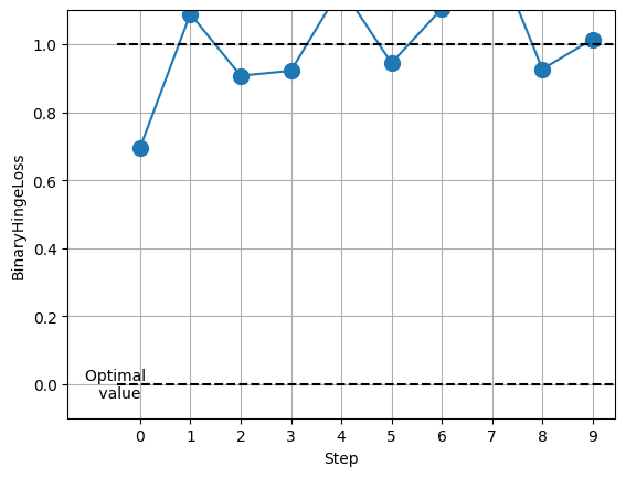
fig_, ax_ = metric.plot(values)
The above code:
- Uses the torch library to import the rand and randint libraries for building the dataset randomly using the for loop.
- Calls the BinaryHingeLoss() method in the metric variable and builds the values from the input and predicted dataset.
- After that append the values to plot them on the graph as displayed on the screen:
That’s all about the process of calculating the hinge loss in PyTorch.
Conclusion
Hinge loss is calculated for the classification models in deep learning and PyTorch offers multiple methods to calculate the loss value. Importing torchmetrics enables the user to implement the HingeLoss(), HingeEmbeddingLoss(), and BinaryHingeLoss() methods. The functional dependency of the torch library can also be used to calculate the hinge loss for multiclass model evaluation. This guide explains all the possible methods of calculating the hinge loss in PyTorch. The guide also implements an example that creates the model for its evaluation and optimization in the PyTorch environment.