The SORTN() Function in Google Sheets helps us find the top-most or the lowest-most entries in a particular data. For example, if you are a business owner and want to see the top three best-selling employees of your organization. With less data, it is easy to find out the top entries, but when we are dealing with hundreds or thousands of entries, there is a greater chance of getting errors in our calculations.
In this scenario, the SORTN function in Google Sheets did this job without getting any errors. From this guide, you will understand/learn in detail how to execute the SORTN function in Google Sheets.
What Does SORTN() Function Do in Google Sheets?
The SORTN() function is a little bit complicated as it accepts several arguments. But nothing to worry about! We will discuss all the arguments used in the SORTN() function one by one. The following is the syntax used for the SORTN() function:
SORTN(range, [n], [display_ties_mode], [sort_column], [is_ascending], [sort_column2, ...], [is_ascending2, ...])Where,
| Argument | Use |
| range | The data you want to sort out to find the top entries |
| n | This is an optional argument, and by default, its value is 1. It is the number of rows you wish to return. For example, if you wish to return with the top 3 rows of the data, then its value will be 3 |
| disply_ties_mode | This is also an optional argument, and by default, its value is zero. It is used to show how many tie items appeared in the first n items. Its value must be from 0 to 3.For 0, you will return with the first n items from the selected range of the data. For 1, it will return with the top n number of rows in addition to their tie entries from the range.For 2, it will show the top n number of rows after removing the ties from the range.For 3, it will show the top n number of rows with their tie. |
| sort_column | It is the optional argument used to include the column to sort out the range |
| is_ascending | This argument is used to sort the data in ascending or descending order. To sort the data ascendingly use TRUE and to sort data descendingly use FALSE as the parameter. |
| sort_column2 | This optional argument is used to include the additional column to sort out. |
| is_ascending2 | This optional argument is used to sort the data ascending or descending from the additional column |
How to Use the SORTN() Function in Google Sheets
Consider the following example with data on a sales report, on which we will use the SORTN() function. This will help in better understanding all the parameters utilized in the stated function.
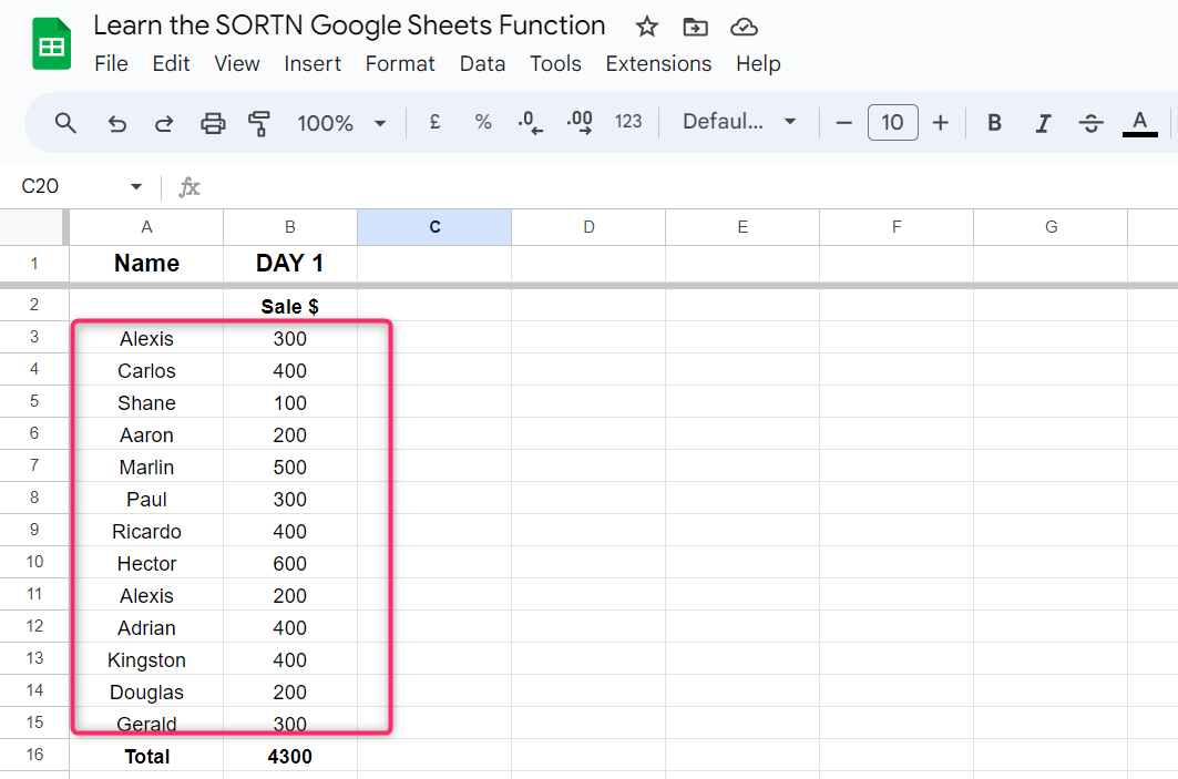
We will learn all the aspects of using the SORTN function step by step.
Step 1: Type the SORTN() Function
Click on an empty column and type =SORTN. As soon you start typing the formula, Google Sheets provides you with a list of the formulas starting with the keywords you type. It’s better to pick the formula from the suggestion list to avoid any mistakes:
Step 2: Type the Data Range
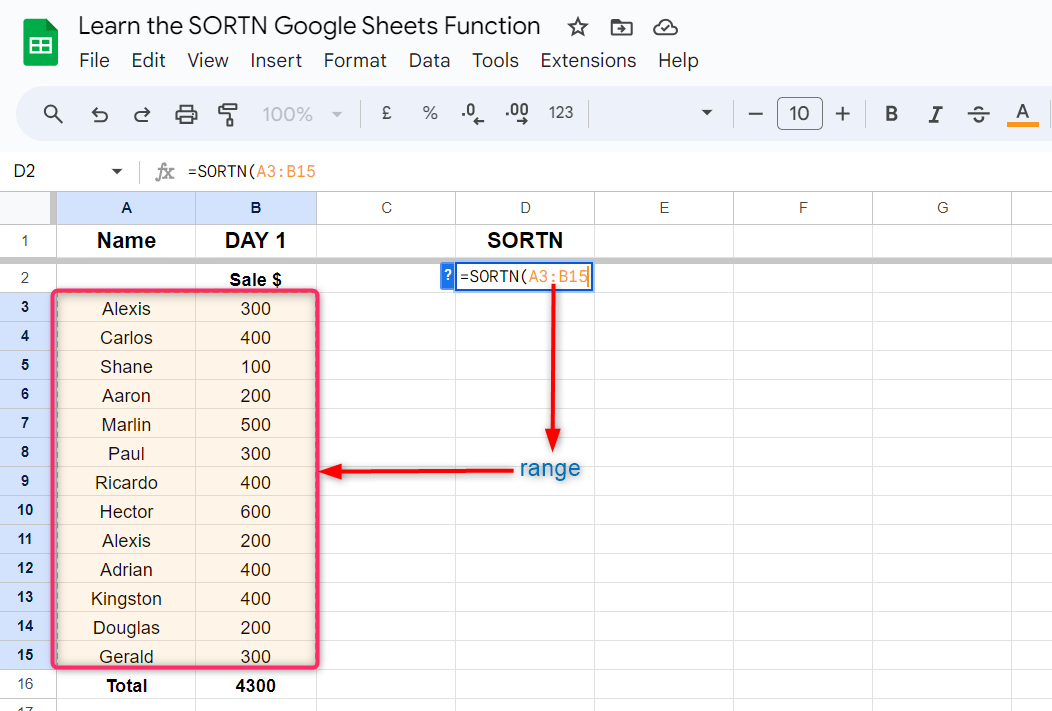
Type the range of the data you wish to sort in. In our scenario, we select/specify the range as A3:B15.
Here, A3 and B15 are the minimum and maximum ranges of the selected data respectively:
Step 3: Enter the Value of “n” and the “display_ties_mode”
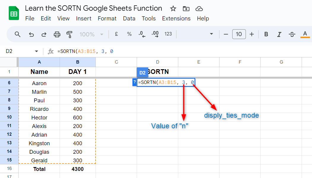
Type the value of n and the disply_ties_mode. Let us choose 3 for n and 0 for disply_ties_mode:
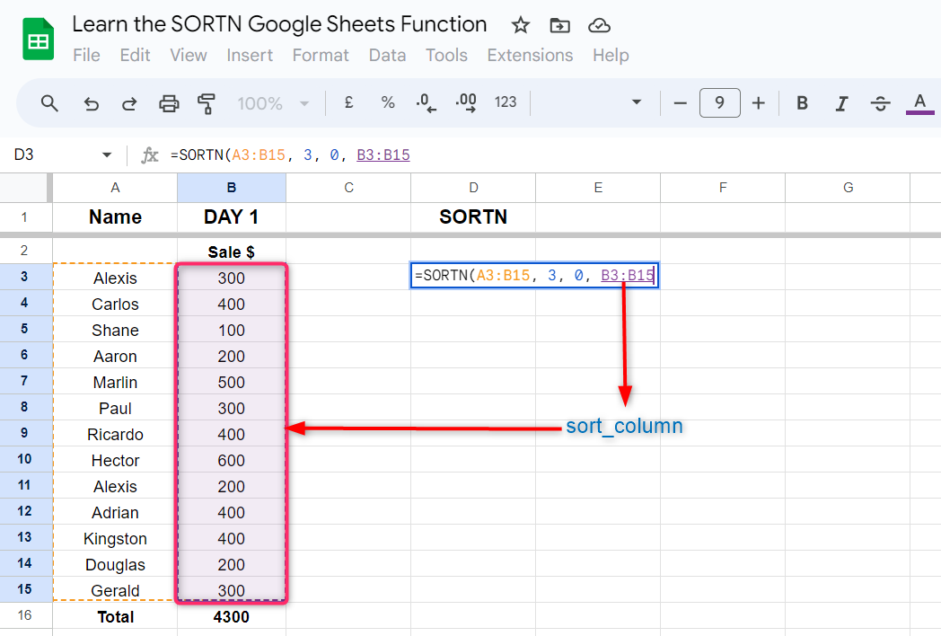
Step 4: Enter Range for “sort_column”
The next argument is sort_column. Enter the range of the column on the basis of which you want to sort out the data. Type the maximum and minimum range of the column manually, or click and hold on the first cell and move the cursor down until the last cell of the range:
Step 5: Type “TRUE” or “FALSE” as the “is_ascending” Argument
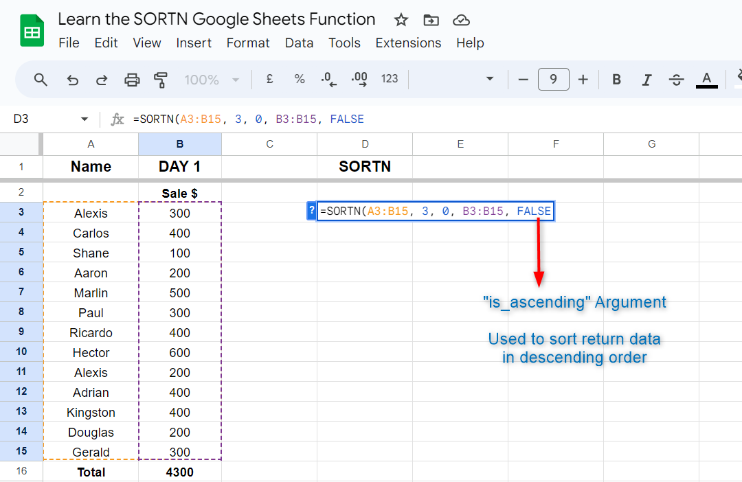
Now, the final argument is is_ascending, which we will use to sort the data in ascending or descending order. Type TRUE to sort the data ascendingly, or type FALSE if you wish to sort the data descendingly.
In our example, we will use FALSE to sort the return data in descending order so that we can easily figure out the top entries:

Step 6: Press Enter
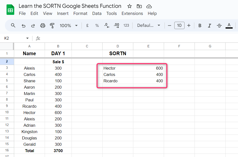
After typing all the required arguments in the SORTN() function, press Enter. We will get the top three positions in the selected data:
Example 2: Use “display_tie_mode” as 1
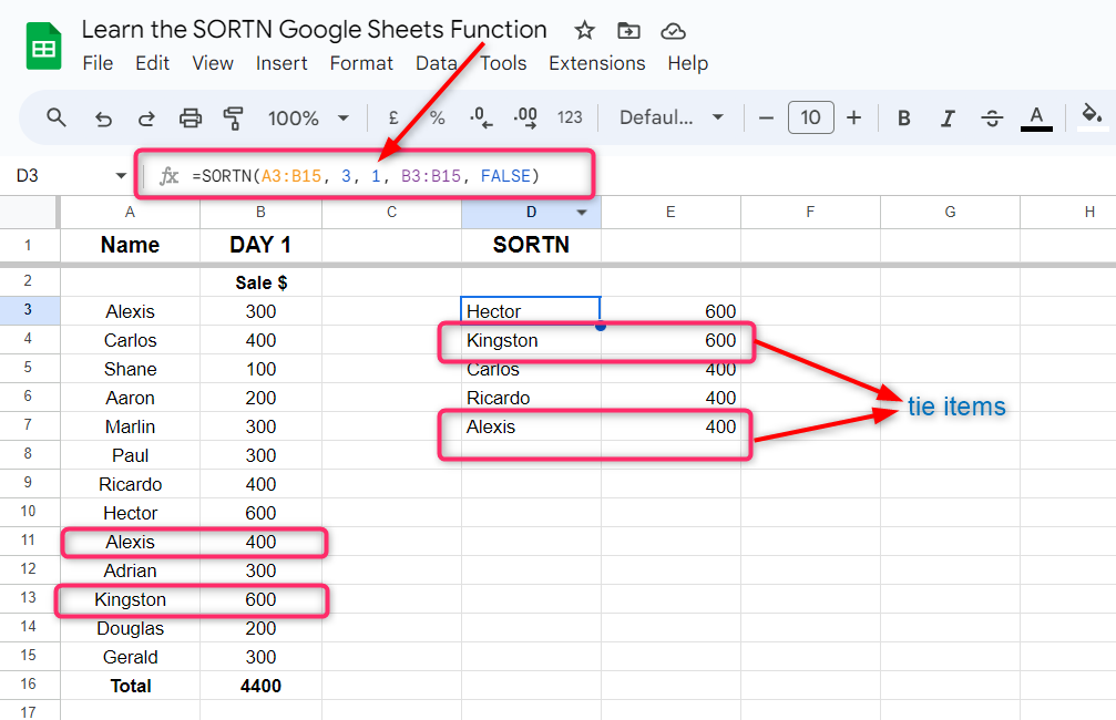
In the same above example, if we use 1 for the disply_ties_mode, then we will get the first 3 rows and, in addition, all the tie rows with the first 3 rows as follows:
Example 3: Use “display_tie_mode” as 2
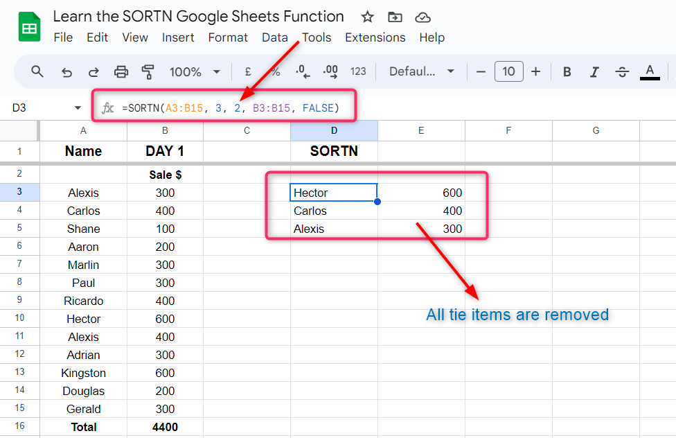
In the same above example, if we use 2 for the disply_ties_mode, then we will get the first three rows after removing the tie rows as follows:
Example 3: Use “display_tie_mode” as “3”
Now, type 3 as the disply_ties_mode in the above example, we will get the first three rows including all the tie rows with them as follows:

Conclusion
The SORTN() function in Google Sheets is a very useful statistical formula to find out the top-most entries in a given data. The SORTN() function is one of the largest functions in Google Sheets, having five arguments. First is the range of data to sort out and then the number of items n.
Third, the display_tie_mode is the most important argument, its value is between 0 and 3 depending on how we deal with the tie items in the data. The fourth is the column selection on the basis of which we sort the data, and the last one is for sorting the return data in ascending or descending order.