The data validation feature in Google Sheets allows the user to control what to type in the cells. You can set up specific rules for the entries in the cells, moreover, data validation allows the user to display a custom message when you enter a wrong value in a cell. In this guide, we will discuss the use of data validation in Google Sheets with practical examples.
How can We Use Data Validation in Google Sheets
Data validation is a quick way to check data in Google Sheets for errors and to ensure that the data meets the standard requirements. For example, if you are a school teacher, and you want to create a report of a test having a total of 25 marks. While creating the report, you are limited to entering the marks between 0 and 25. Any entry greater than 25 and less than 0 is invalid.
Following is the list of some data validation rules, we will discuss each of them one by one in detail with examples:
- Set Data Validation Using Number Limit in Google Sheets
- Set Data Validation by Creating a Dropdown List Google Sheets
- Set Data Validation by Adding a Custom Formula in Google Sheets
- Set Date Validation Using Data Validation in Google Sheets
- Set Data Validation Using Text Rule in google Sheets
1: Set Data Validation Using Number Limit in Google Sheets
In the number limit validation rule, we add a condition for the numerical values to be added in the data. For example, in the data of test results, if the total marks are 60, then we can set the data limit to be between 0 and 60. Any value greater than 60 and less than 0 will be pointed out and show a warning text against this value. Below are a few steps to add a number limit in Google Sheets.
Step 1: Select Data
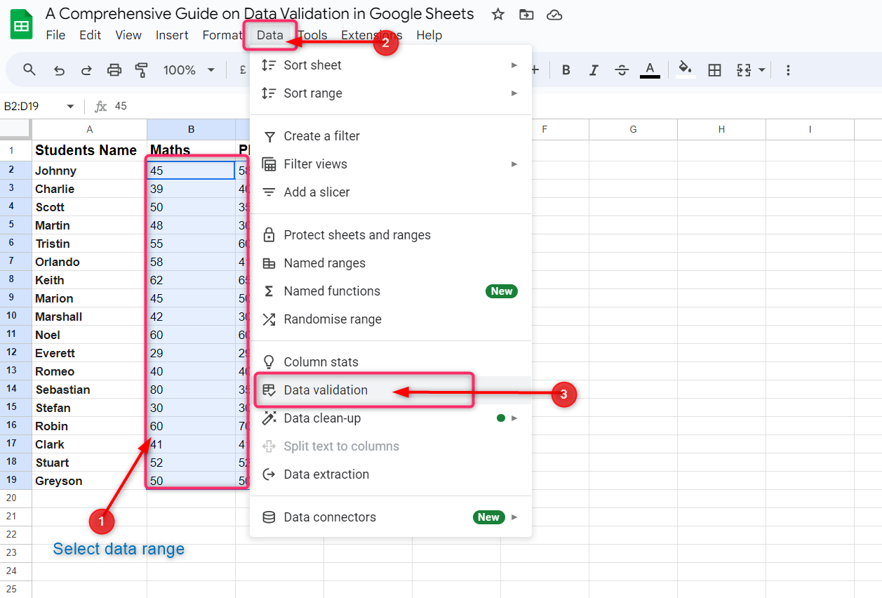
Select the data range on which you would like to apply the number limit and click on Data from the taskbar and then from the context menu click on Data validation:
Step 2: Add New Rule
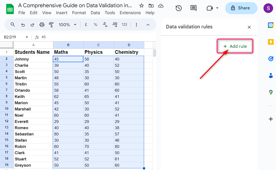
Under the Data validation rules, click on Add rule:
Step 3: Select a Number Rule
Click on the box under the Criteria to select the number rule you want to apply to the selected data range:
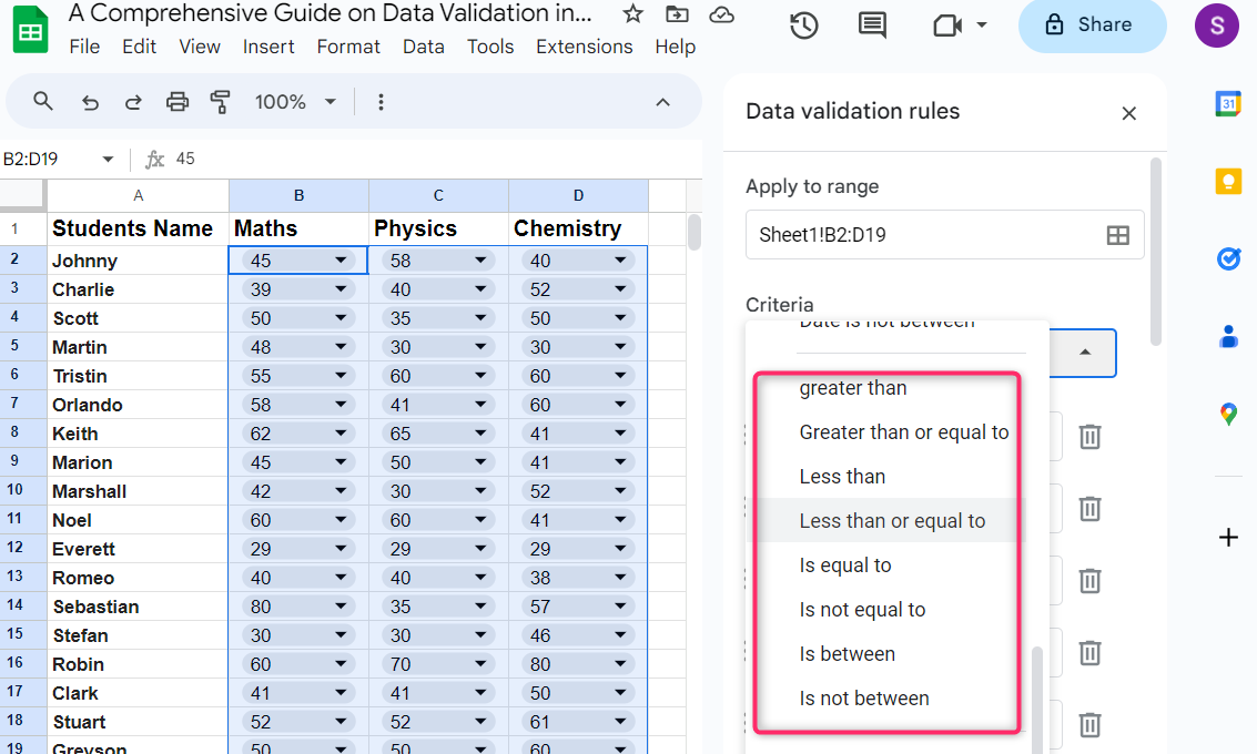
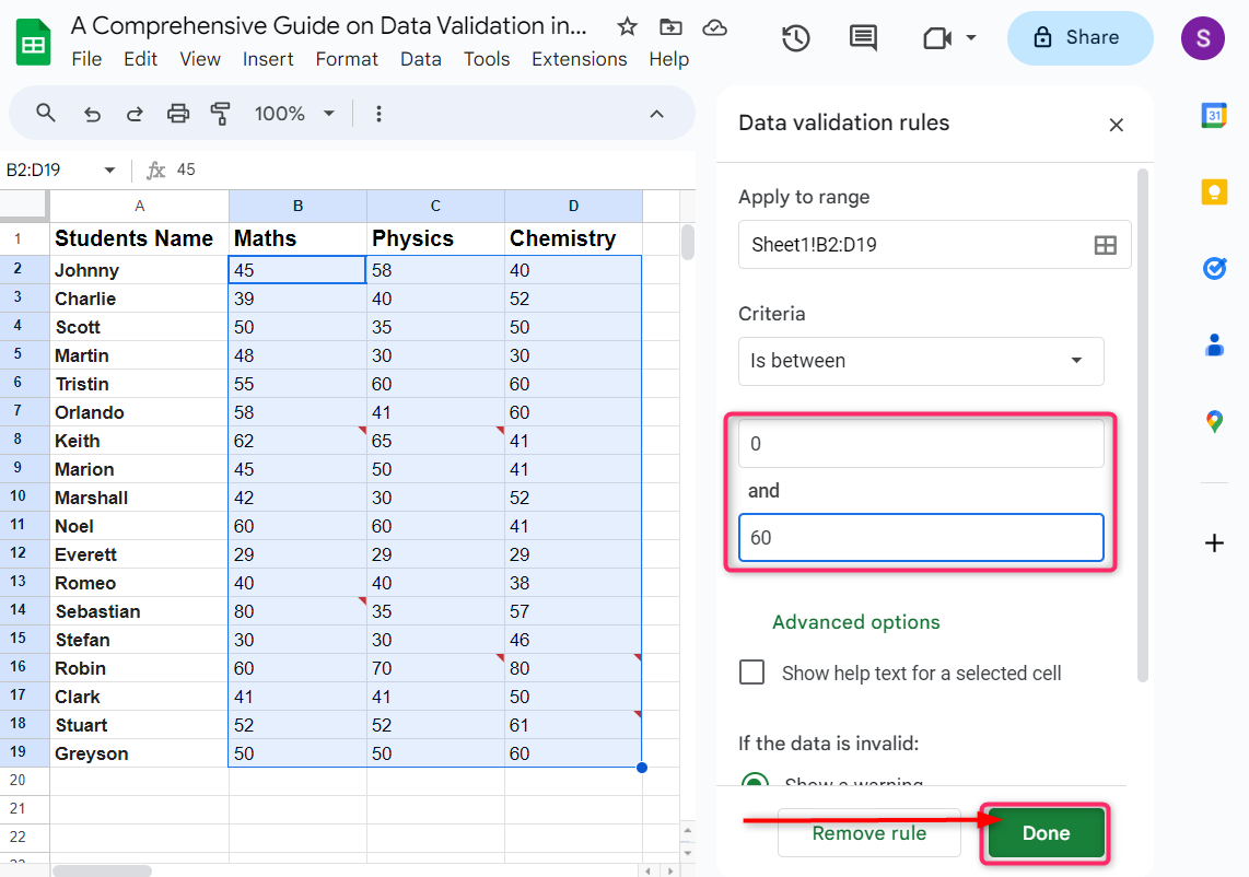
In our example, we will select In between as a number rule to apply to the selected data:
Step 4: Add Number Limit
New boxes will be added under the Criteria. Type the minimum and maximum number limit you want to set as a number rule and click on Done:
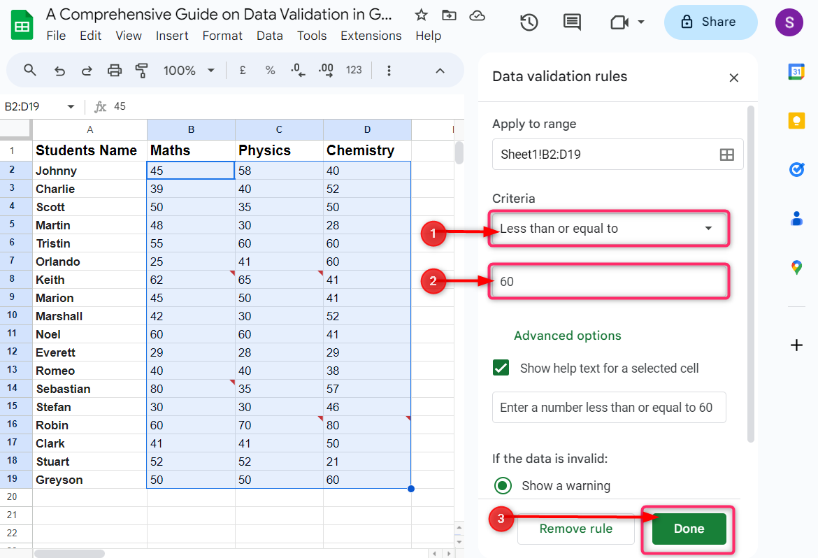
In the same example, let us choose Less than or equal to option under the Criteria and enter 60 in the conditional box, then click on Done. This will only accept the entries that are less than and equal to 60 and show warning text to the entries greater than 60 as invalid entries:
2: Set Data Validation by Creating a Dropdown List Google Sheets
In the dropdown data validation rule, we can only put the values or text available in the dropdown. By creating a dropdown list of values or texts, there is no chance of adding inappropriate data, as we can only choose data available in the dropdown. There are some simple steps to follow to create a dropdown list with data validation in Google Sheets.
Step 1: Create a Dropdown for Selected Data
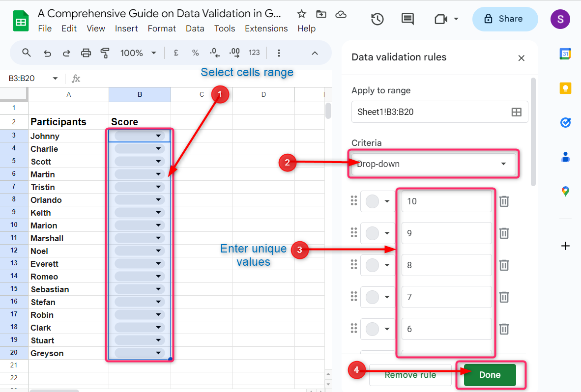
Select the cell range on which you want to create a dropdown list and go to Data validation rules as mentioned above. Under the Criteria, select the Drop-down from the options and type the unique value you want to add to the drop-down list in the boxes next to the criteria. Once you added all the required items in the drop-down list, click on Done:
Step 2: Assign Colors to Dropdown Items
We can also assign different colors to each item in the drop-down list. To assign colors to the items in the drop-down list, click on the boxes with a small circle next to the drop-down items boxes and assign them from the available colors.

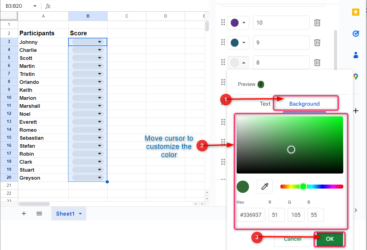
To assign a customized color to an item in the drop-down list, click on Customise below the available colors.
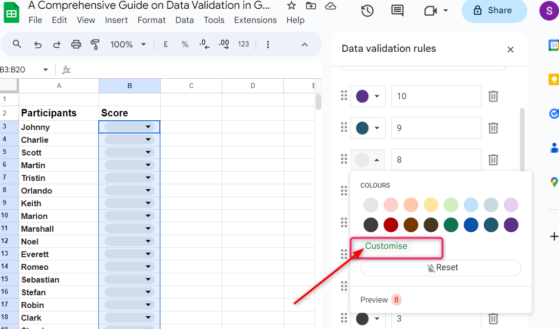
Customize the color by moving the cursor on the color box and color slider. Once you customize the desired color, click on OK to assign it to the selected item:
Step 3: Apply Dropdown Items
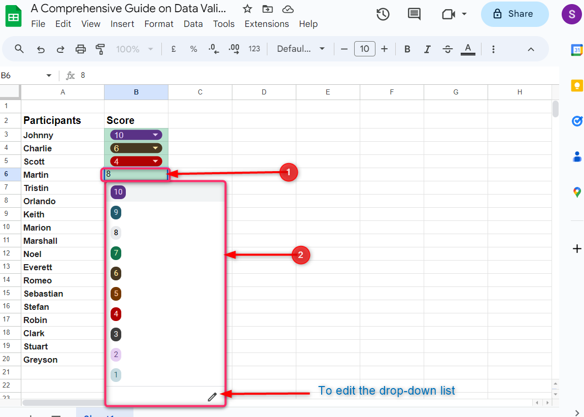
Now click on the boxes in front of the student’s name and give ranks to the students from the drop-down list you have created with the colors. You can edit your drop-down by clicking on the pencil icon at the bottom of the list:
3: Set Data Validation by Adding a Custom Formula in Google Sheets
To apply the custom formula using data validation in Google Sheets, select the data range and go to data validation rules as mentioned above.
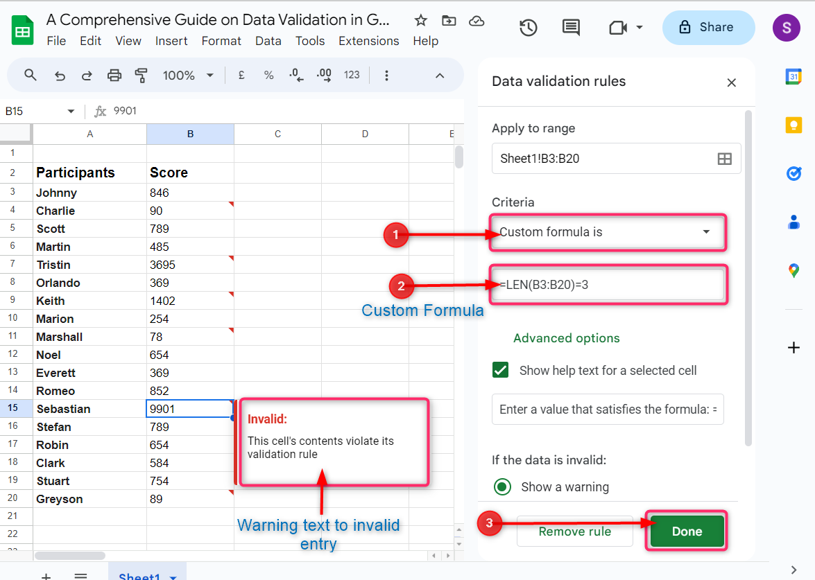
In data validation rules, click on the box under the Criteria and choose Custom formula is from the dropdown options. A new box will be added next to it to add a formula. Enter the required formula and click on Done.
In our example, we added the formula to restrict the values in the data with 3-digit numbers only. Any entry with less or greater than three digits will never be accepted:

4: Set Date Validation Using Data Validation in Google Sheets
Using Data validation in Google Sheets, we can set a date limit to check whether the entry is valid or not. Consider an example to better understand this feature, students are asked to submit their assignment before 15/09/2023. If any students submit the assignment after the submission date, Google Sheets will point out the entry with a warning text as an invalid entry. Following are a few steps involved in setting up a date rule in Google Sheets.
Step 1: Select Criteria
To set the date limit in the Google Sheets, open the data validation rules as mentioned above and select a date validation rule from the drop-down under the Criteria.
There are eight different date validation rules, and you can choose any of them according to the date limit you want to assign to the data:
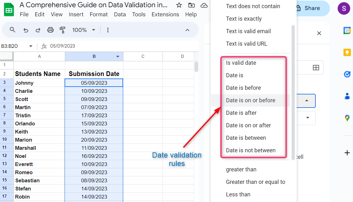
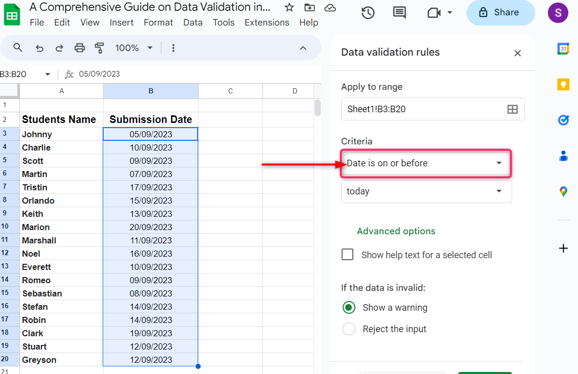
In our example, we choose the Date is on or before:
Step 2: Select a Date Rule
As soon as you choose the date rule, a new box will be added next to it. Click on this box and select the date you want to set from the drop-down:
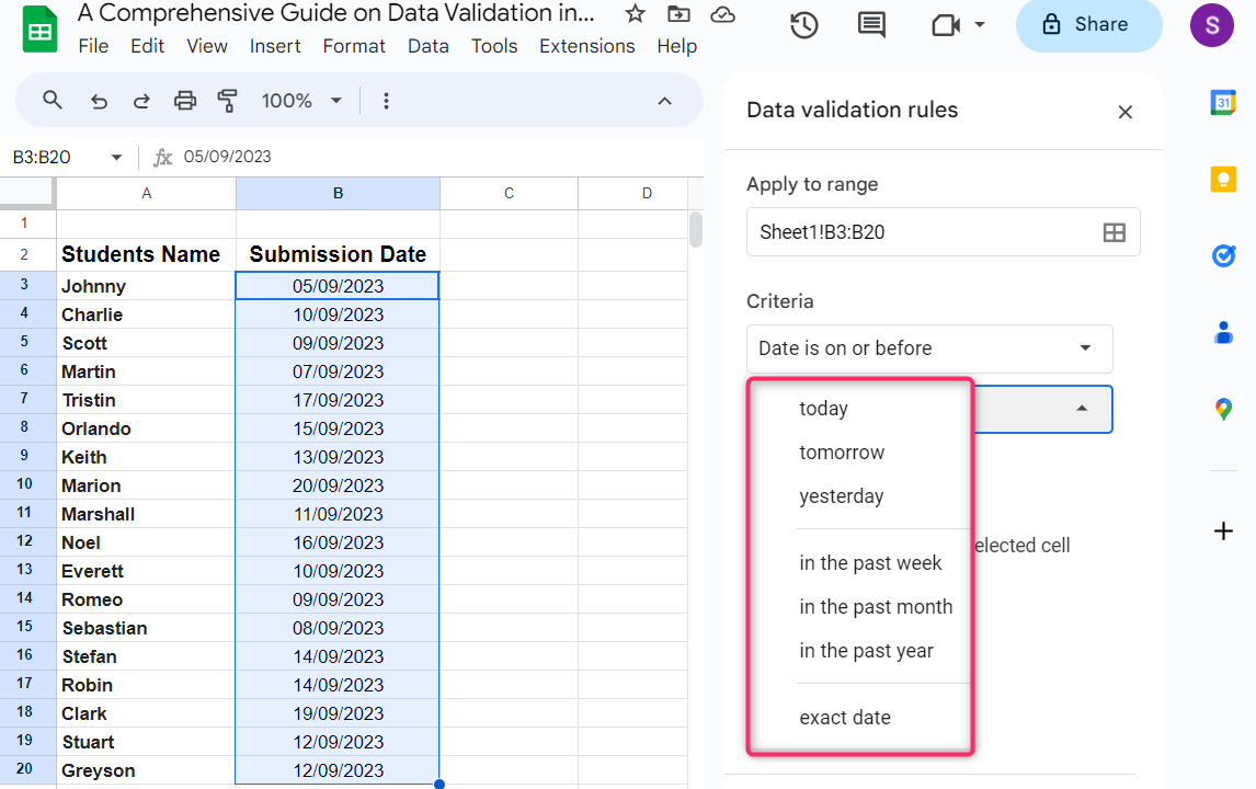
In our example, we will choose the exact date to set the date limit manually:

Step 3: Type the Date Manually
There will be a new column added under the Criteria. Type the date you want to apply to the selected date range and click on Done. This will accept the entries before and on the date, which is 15/09/2023, and show a warning text to the entries after this date as invalid entries:
There will be a new column added under the Criteria.

5: Set Data Validation Using Text Rule in Google Sheets
We can also set a text rule to apply to the data in Google Sheets to check if the entries are valid or not. To apply the text rule, select the data range and go to the data validation rules, as mentioned above.
Step 1: Select Criteria
Click on the box under the Criteria and select the text rule from the drop-down menu:

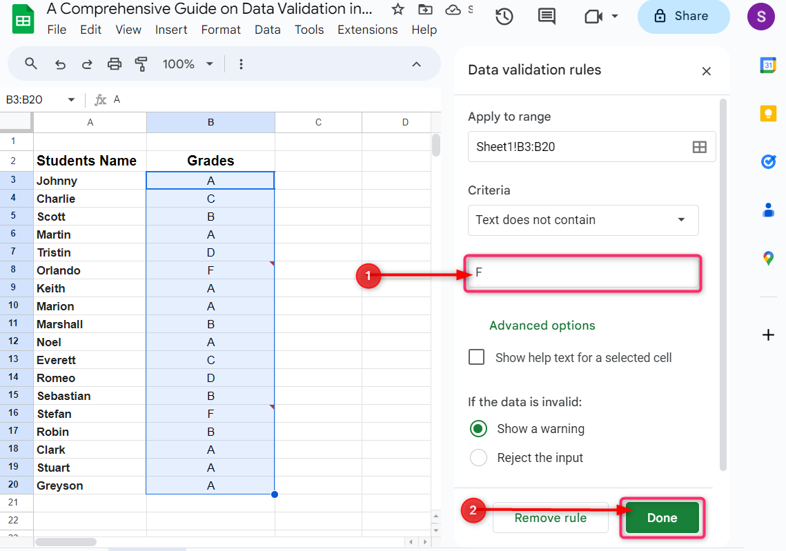
In our example, we will select Text does not contain as a text validation rule:

Step 2: Type Text Rule and Apply
A new box will be added next to it. Type the text here that you don’t want to contain in the selected data range and click on Done:
Conclusion
Data validation in Google Sheets is used to check the data for errors to ensure it meets the standard data requirements or not. Using the data validation feature we can set a number limit, make a drop-down list of unique entries, set a date limit, create a custom formula, and set a text validation rule. Select the data range, click on Data from Google Sheets’ taskbar, and click on Data validation from the drop-down. Under data validation rules, click on add a new rule. Under Criteria, select the rule you want to apply and follow the instructions next.